My introduction to Bayes
I now consider myself a software engineer, but my journey into programming started with an interest in probability and uncertainty.
In the early days I was doing little experiments in spreadsheets, bumping around in a dark room without much ability to navigate. Around the same time I also started getting exposed to blogs like Less Wrong and the writings of Eliezer Yudkowsky—who, incidentally, is currently sounding the alarm that superintelligent AI is going to literally kill everyone if we build it—but this post isn’t about existential dread, or the mentally unmooring effect of having one of your foremost intellectual influences prophesying imminent doom.
Less Wrong and Eliezer introduced me properly to Bayes. I say properly, because reading a Wikipedia article or having professors gleefully show how “unintuitive” it is, is about the worst way you could possibly be introduced to it. These writings were not gleeful in challenging intuition, but patient and aphoristic, teaching by example through excellent technical writings, rather than whiteboard problems.
Bayes intersected with my work, and my interest in uncertainty, so these influences came together at a great time in my career.
More importantly, the introduction to Bayes was a formalized introduction to rationality and probabilistic thinking in general, which for whatever reason I am very predisposed to, and following that rabbit hole led me to Bayesian statistics.
This led me to dig for more influences, like E.T Jaynes, Aubrey Clayton, Cameron Davidson-Pilon’s Bayesian Methods for Hackers and the incredible work (in lectures and textbooks) of Richard McElreath.
Bayesian statistics required me to program, so I learned, and on the way learned that my home was always going to be in software engineering, I just hadn’t landed on that path yet. So Bayesian statistics, in the end, is the reason I am doing what I’m doing today.
And software engineering combined with Bayesian statistics is a very powerful combination, as it turns out.
Because I’m not a formally trained statistician (or an academic of any kind), but instead someone who works in a technical industry where engineering and data analytics are highly valued, my perspective on where Bayes fits in is as much value-oriented as it is driven by intellectual curiosity. I’ve written before about the idea of informatics, and Bayesian statistics sits at the heart of the concept.
The point I want to make in this post boils down to this: the Bayesian toolkit lets us combine domain knowledge and limited data into highly expressive, interpretable models that quantify uncertainty, and this makes them ideal for decision support in complex technical domains.
The core of it
A. “What should we believe, given our understanding of the world and our data?”
B. “What should we do, given that information?”
Bayes helps us define what to believe, decision theory formalizes what actions to take, and our values ultimately decide what we do.
In contexts where decisions are difficult, uncertainty is an essential ingredient. You really can’t make good decisions in the absence of a consideration of uncertainty—we do it all the time by calling options “safe bets” or “high-risk”—probability models just quantify these considerations and make them explicit.
The uncertainty is ultimately subjective (all probabilities are in the Bayesian view), but subjective quantities still follow rules. If you want to trace your uncertainties through to their logical consequences, you need to obey those rules.
Monte Carlo models
Monte Carlo models are the first thing to master when learning how to use probability. They are incredibly flexible and simple in concept. Define your uncertainties, state the math that governs the outputs you care about, and run the system thousands of times to see what happens.
You can teach yourself a lot by doing this. You will discover SEM by adding stochastic outputs together. You will quickly disabuse yourself of mental mistakes relating to “stacking percentiles” because you can watch the real result occur in simulation. You will understand CDFs and PDFs and quantile ranges without even knowing their names, because you will understand that behind everything is an array of simulated values, not a mysterious system of mathematics that is beyond your understanding.
You can start doing this without even understanding the probability distributions in the background—that understanding will come as you delve deeper.
Back of the envelope thinking
In The Art of Doing Science and Engineering by Richard Hamming, he talks about the usefulness of back of the envelope problem solving. Modern computing gives us the tools to take back of the envelope problem solving into the probabilistic realm with minimal effort.
One of Hamming’s examples is the idea that (back when he wrote the book in the late 80s) 90% of the scientists who have ever lived are now alive. He takes that statement along with an assumption that knowledge doubles every 17 years, to do a back of the envelope calculation to see how compatible the two statements are.
I will skip the maths (apparently integral calculus was part of Hamming’s idea of back of the envelope thinking), but he shows that if the number of scientists practicing at any time is given by:
\[ y(t) = ae^{bt} \]
and, assuming scientists have careers lasting around 55 years, the proportion alive today is given by:
\[ 1 - \left(\frac{1}{2}\right)^{55/17} = 0.894... \]
And he makes the point well. Comfort with turning claims into a bit of maths allows him to test assumptions with minimal effort, and in this case he is left satisfied that the claims are consistent.
Modern computing and tooling means that for us, with a laptop and a Python install, we can add our uncertainty to the mix with minimal effort. Say we think the doubling time is centred on 17 years, and the length of a scientist’s career is centred on 55 years, but we’re uncertain about both quantities:
import numpy as np

n = 5_000

rng = np.random.default_rng(42)
career_years = rng.normal(55, 10, n)
doubling_years = rng.normal(17, 3, n)

proportion_alive = 1 - (1 / 2) ** (career_years / doubling_years)
Mean result: 0.883; 90% interval: 0.763–0.968Maybe we care about this uncertainty, maybe we don’t, it depends on the problem and the stakes. The point is that it is incredibly easy to do, and now with AI, all that is stopping you is a passing familiarity with the concepts, and just asking!
Scale to any problem
Monte Carlo models can be self-contained and simple, like the above example, or they can get arbitrarily complex, but the style of thinking that makes it clear how this trick is done is all you need to start. You will pick up more complex concepts like multivariate correlated sampling, working with high dimensional arrays, and vectorization as you delve deeper, but the core framework is incredibly simple to start with.
Just make the computer go brrrrrr.
Learning from Data
It might appear that I’ve diverged from the point of this post (using Bayes to solve technical problems and improve decision making) but the Monte Carlo method is a good entry point, because it begs a question:
How do we decide what distributions to use? And how do we parametrize them?
Formalizing uncertainty in a Monte Carlo model is great, but how can we be rigorous about the parameters that define the distributions that model that uncertainty?
In the example above I set the length of a scientist’s career to \(\text{Normal}(55, 10)\)… but I just pulled that distribution out of a hat.
In Bayesian statistics terms this would be called elicitation. We ask someone what they think is a reasonable range of values for a particular quantity (before looking at any data) and we take their answer and “elicit” an appropriate distribution that captures that belief.
But there is no data here, how do we take that prior belief about the quantity and use data to learn about it?
That requires Bayes.
\[ p(\theta \mid y) = \frac{p(y \mid \theta)\,p(\theta)}{p(y)} \]
The left side of that equation means, in words, What is the posterior probability distribution over the model parameters, given the observed data, which sounds similar to
A. “What should we believe, given our understanding of the world and our data?”
In technical contexts these are the same thing, because our beliefs are formalized by the parameters in our Monte Carlo models.
So now we’ve added data (\(y\)), how do we use it in practice?
The field of Bayesian statistics is devoted to this problem.
Markov Chain Monte Carlo models
It turns out that Bayes theorem is a huge pain in the ass. There are classes of problems where the maths work out elegantly, providing efficient analytical solutions to Bayesian models. These are very cool and useful to learn, but also rare when applied to real-world problems.
Most of the time, we need specialized algorithms to do Bayes. It is all because of this innocent looking probability in the denominator of Bayes theorem:
\[ p(y) \]
Which equates to
\[ p(y) = \int p(y \mid \theta)\,p(\theta)\,d\theta \]
“The denominator is the probability of the observed data under the whole model. It integrates over every possible value of \(\theta\), weighting each value by its prior plausibility. In other words, it asks how surprising the data would be before we knew which parameter value was true.”
That sentence is a headache. I actually asked the AI to write it because I couldn’t manage a sentence describing it.
It turns out it is a headache for computers, too, because most of the time that integral is an intractable nightmare, where no analytical solution even exists.
Instead, clever algorithms are needed to approximate the posterior distribution through random sampling. This is Monte Carlo again, but this time we have no way of sampling the distribution directly, because it is unknown, so we have to explore the probability space without it, somehow. That is where Markov Chain Monte Carlo (MCMC) algorithms come in.
Learning how to build efficient models to do Bayesian inference is the engineering side of Bayesian statistics.
This isn’t a post about that engineering effort, but the point is, with MCMC models, we can update our beliefs with data across a wide range of problems.
What about Machine Learning and AI?
The dominant paradigm in data science is machine learning. Many mainstream machine learning workflows are built around optimization: choose a model class, define a loss function, and find the parameters that make the best in-sample predictions while minimizing out-of-sample error. For big datasets with many features, this can work incredibly well.
But running problems through the black box of ML costs us a few important things.
First is expressiveness. Engineering problems usually have an underlying mathematical structure that is well understood. It is not wise to throw it out and expect the algorithm to pick it all up again using large quantities of data. Physics informed neural networks (PINNs) address this problem, embedding physical laws into neural network training such that solutions are kept within physically consistent constraints, but they are not the norm in the ML world—most of the time ML models are not constrained in this way.
Second is uncertainty. Most machine learning algorithms do not provide uncertainty quantification. Especially in complex domains with limited data, that uncertainty can be an essential component of effective decision making. In high stakes situations, an ML model stating that the answer is “25!” while not having any ability to provide confidence intervals of \(\pm 10\) or \(\pm 1000\) makes decision making based on their results far less robust.
Third is what I call the problem of “small data”. Big data is a luxury that most engineering problems don’t enjoy. Instead we are often trying to maximize the information we can get out of small quantities of expensive-to-acquire data. Machine learning solutions in this context are not the best choice, in my view. They will provide uninterpretable solutions with questionable validity, with no uncertainty preservation.
Machine learning is a rich field with many answers to the issues I bring up here, but my answer is: use Bayes instead. I think it provides a better toolkit in many engineering contexts.
Examples
I want to show a few examples here. My background is in oil and gas, so that is where I know problems in the most detail, but I want to stress how domain-agnostic Bayesian statistics is. If you have a system of equations that govern behaviour in some domain you are studying, you can express it in a Bayesian model, feed it data, and do inference.
These examples all follow the same pattern. It is a playbook that can be adapted for any technical domain:
- start with an engineering calculation or domain relationship,
- represent uncertain inputs as probability distributions,
- define prior beliefs over those inputs through discussions with domain experts,
- use Bayes to update those distributions with data where it is available,
- propagate the resulting uncertainty into a decision-relevant output.
I should stress that this is a gallery of examples, more than a rigorous working of each problem, and all use synthetic datasets. They are snippets of more nuanced problems that oil and gas technical workers face, used to communicate how Bayes can help.
These models are created and run with PyMC, a popular Python package for doing Bayesian statistics.
Oil Field Volumetrics
A classic petroleum engineering example is a volumetric estimate. The deterministic calculation is simple, but every input is uncertain: porosity, water saturation, net to gross, gross rock volume, and the oil formation volume factor. Offset wells can teach us about reservoir properties, while other properties are derived from separate studies, like geophysics-driven structural modelling, or PVT-driven formation volume factor calculations.
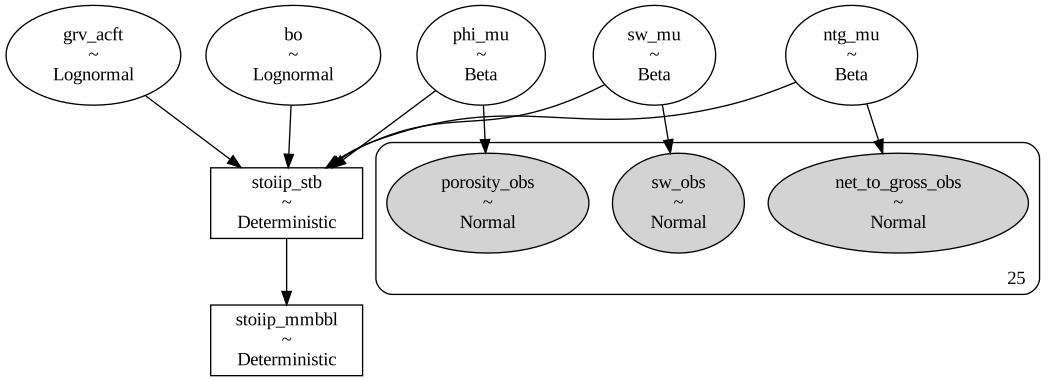
The following is a simple PyMC model using synthetic offset-well data. The 25 wells inform field average porosity, water saturation, and net-to-gross. The formation volume factor, \(B_o\), and gross rock volume, GRV, are included as priors with no direct observations. STOIIP is then calculated as a deterministic variable from posterior samples of the reservoir parameters.
Here is a sample of the (synthetic) data:
| well | porosity | sw | net_to_gross | |
|---|---|---|---|---|
| 0 | W-01 | 0.217618 | 0.315915 | 0.440238 |
| 1 | W-02 | 0.184000 | 0.351292 | 0.464190 |
| 2 | W-03 | 0.228761 | 0.344618 | 0.317999 |
| 3 | W-04 | 0.233514 | 0.346509 | 0.397623 |
| 4 | W-05 | 0.161224 | 0.347233 | 0.387074 |
Here is a graph representation of the statistical model. Grey nodes indicate observations (data), and white nodes are latent (unobserved) model parameters:
And here is the result:
Here I’m showing the prior STOIIP (the distribution that the subsurface team might have estimated before discovering this field), and the well-data-driven posterior STOIIP, which has converged on a tighter uncertainty around the true value as the offset-well data updates the field-level reservoir properties.
The point of putting the volumetric equation inside the probabilistic model is that the STOIIP output is not a separate spreadsheet calculation bolted on afterwards. It is part of the model graph. The same samples that update porosity, water saturation, and net-to-gross from the offset wells also propagate the prior uncertainty in GRV and \(B_o\) into the final volume estimate.
Making the STOIIP part of the model graph also makes some advanced modelling possible, like integrating observed production as an additional constraint. If 4 MMSTB had already been recovered from this reservoir, for example, it would indicate STOIIP values less than ~8 MMSTB are highly unlikely, as recoveries of greater than 50% in oil reservoirs are uncommon.
Fluid contact uncertainty from RFT data
Another fun example in the oil and gas context is estimating fluid contacts based on pressure points taken in reservoirs. One can infer the depth of a gas-water contact based on this data, but it is often an uncertain estimate due to unknown fluid properties like the salinity of the brine (water) and the density of the gas. The water gradient is also often far less well sampled than gas columns.
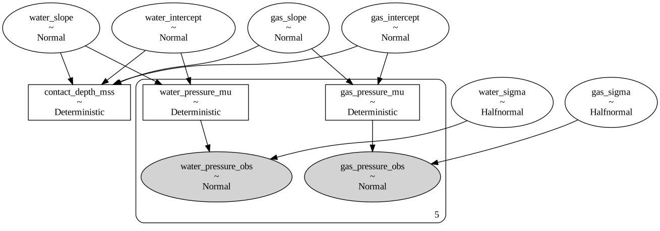
The problem boils down to finding the intersection of two lines: the gas pressure gradient and the water pressure gradient. The intersection of two lines is computable as:
\[ \begin{aligned} y_1 &= m_1 x + b_1 \\ y_2 &= m_2 x + b_2 \\ x^* &= \frac{b_2 - b_1}{m_1 - m_2} \\ y^* &= m_1 x^* + b_1 = \frac{m_1 b_2 - m_2 b_1}{m_1 - m_2} \end{aligned} \]
If we can model those pressure gradients with a Bayesian statistical model, we will also get full uncertainty quantification for the pressure and (of more interest) the depth of the intersection, which represents the gas-water contact.
Let’s start by simulating some data:
Each pressure gradient is a linear function, so our Bayesian model is simply estimating the slope and intercept of each, then passing the solution for their intersection into the model graph to output it as an uncertain parameter.
Fitting the model to the data yields our two pressure gradients:
And the uncertain intersection of those two lines is the uncertainty in the contact depth, also shown below as a histogram:
Neat!
Now this range can be used when assessing trapping geometries, whether through showing a range on a single depth map, or simulating depth map iterations with this uncertainty fed in. This may have a dramatic effect on volumetric estimates, depending on how sensitive the trapping geometry is to changes in the contact.
Fluid compositional modelling
A Dirichlet model can be fit to a dataset of fluid samples to model uncertainty in composition across a field. This example benefits from hierarchical modelling (a Bayesian statistical superpower) to account for groupings of data, like replicate samples of the same interval, or samples from the same reservoir.
Again, we start with some synthetic data:
Note these are the average compositions of the three reservoirs; in reality we have several fluid samples (and replicates) in a dataset of 21 total samples.
So how can we model the average properties by reservoir, and the variability we see within sample intervals and across them?
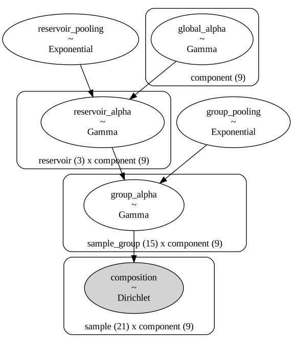
A hierarchical or multi-level model allows for information to flow between observation groups. Here we are trying to learn about the average compositions of samples collected across a field, from particular reservoirs, with repeated observations over some intervals. That leads to a natural field-to-reservoir-to-sample-group hierarchy.
Intuitively we know that replicate samples from the same interval should be clustered more tightly than samples from different reservoirs. The hierarchical model reflects this. Information flows from the global (field) level, down to the reservoir level, down to the sample group level in a kind of prior pass-the-parcel in the model. This regularizes estimates across each group, so that the bias caused by a naive arithmetic averaging approach over repeated samples is removed from the statistical estimate.
The Dirichlet distribution is useful here because it is a distribution over the unit simplex. This just means that a sample from the distribution generates a vector of values that sum to 1, which matches compositional data nicely. In real examples there would be additional mole fractions included, but I’ve left them out here for the sake of keeping plots readable.
A model like this may become of particular interest while investigating if two reservoirs are in pressure communication. Sparse information, a hierarchy of sampling, and this model gives an engineer a way of quantifying a probability that directly answers the question, or the number of additional samples needed to answer it conclusively!
Sidewall Core Analysis
Sidewall cores are a very rich dataset that lends itself to hierarchical analyses as well. The cores are taken from particular reservoir intervals in wellbores across a field. Routine Core Analysis provides lab-measured porosity, permeability and saturations, often with sampling error included.
Measurement error is another area that Bayesian modelling really shines. I’ll focus on the porosity for this example, but this can easily be extended to a porosity-permeability model as well.
Again, let’s start by creating a synthetic dataset:
Reservoir A appears to be the highest porosity reservoir in the dataset, with Reservoir B significantly poorer in quality. Lab measurement error is included with each data point.
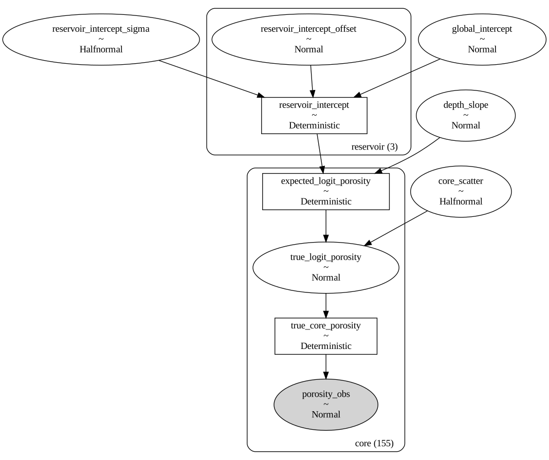
We can fit a hierarchical model with measurement error included to this dataset to model the relationship between porosity and depth for each reservoir.
The model below keeps the depth slope shared across all reservoirs, but allows each reservoir to have its own intercept. Those reservoir intercepts are themselves drawn from a global field-level intercept, giving us a hierarchical structure. The measured porosity values are treated as noisy Gaussian estimates of latent, unobserved true core porosities, with each observation using its own lab-reported sampling error.
We can then visualize the fitted reservoir trends alongside the inferred true porosity for each individual sidewall core:
The vertical tick marks show the lab measurements, while the connecting lines and circular markers show how the model shrinks each noisy measurement toward the posterior mean true porosity implied by the reservoir-level depth trend.
This automatic regularisation is a key benefit of Bayesian modelling. Noisy outliers with high sampling error all receive a posterior estimate that is informed by the linear depth model. The model isn’t asked to do this explicitly, it is just inherent in its structure.
The unintuitive thing about this—which also brings the message home once you internalize it—is that every parameter in the model is being sampled as one facet of a single probability distribution. Each sample’s measurement error is a dimension of the distribution being explored by the MCMC algorithm. That means the system of uncertainty is all tied together by a single estimator, Bayes theorem, over the elaborate multidimensional distribution that our model specifies, which here includes hierarchical pooling, a logit-linear depth trend, and measurement error.
This flexibility and expressivity, and the uncertainty quantification that comes along for the ride, is a big part of the reason why I am so passionate about Bayesian modelling.
Decisions
All of these technical examples derive their value to a business through their ability to improve decision making. As much as I love diving into the rich detail of this kind of work (and doing it well certainly requires that) the point is not the detail, it is the decisions downstream.
Uncertainty as a first-class citizen in business decision making is a key area that I think Bayes can help with.
All of these examples are connected to critical business decisions. Should we drill the prospect? Should we continue developing? How critical is contact uncertainty to our reserves bookings? How can we predict reservoir properties at depths we have not yet explored, and is there opportunity down there?
All of these questions have very uncertain answers, but answers nonetheless. Formalizing the questions as Bayesian models makes this uncertainty explicit, so that decision makers can grapple with it directly.
Technical people often recommend against “confusing” decision makers with rich probabilistic outputs, but I completely reject this. A child can look at two overlapping distributions, presented visually, and tell you about them.1 The problem is in the quality of technical communication, not the lack of understanding in decision makers’ heads.
Bayes does away with flowcharts of different statistical tests and metrics in favor of a single, overpowered output: the posterior distribution. That distribution is about as intuitive an object as statistics can produce—it is just wrapped up in complex language and process, so that it appears scarier than it is—but it is the uncertainty.
And uncertainty is the reality of the situation. It is our responsibility to make that reality clear to the people who are relying on our work to navigate a complex and uncertain world.
While subjective priors may warrant some skepticism, and need to be chosen carefully, the point is that if we agree to the priors, and we model the data, the resulting posteriors are a logical consequence of our beliefs and the data. This is very powerful if internalized fully. Vanilla Monte Carlo models can’t make this claim, as they are not fit to data; they rely on subjective (or optimization-driven) probability estimates.
Bayes instead says “get me started with your prior beliefs, and I’ll tell you how to update those beliefs based on the data you feed me.” That should be music to a domain expert’s ears.
Closing thoughts
Bayesian statistics is certainly not the tool to use in every circumstance, but for me, at least, it was the branch I climbed down from.
These days, spending more time closer to the ground, I still look up at it as my favourite destination, and I visit often.
All my subsequent obsessions, from scripting and software engineering to database design and data engineering, were really pursued in service of that Bayesian ideal of information flowing through to posterior beliefs, and then on to good decisions. Getting all your data in order is absolutely essential to make these systems sing, so it was natural for me to get so into data systems design during my career. Data systems are valuable for all sorts of reasons, but for me it all started with Bayes.
Regardless of the overwhelming cultural emphasis on ML, and now LLM-based AI, Bayesian modelling will always be my favourite reason for having learned how to program, and the toolkit I turn to with the most enthusiasm when the problem calls for it.
Thanks for reading.
Footnotes
I don’t have kids yet. Citation probably needed.↩︎