| Count | |
|---|---|
| Outcome | |
| DHI | HCs (True Positive) | 25 |
| DHI | No HCs (False Positive) | 2 |
| No DHI | HCs (False Negative) | 15 |
| No DHI | No HCs (True Negative) | 30 |
Direct Hydrocarbon Indicators
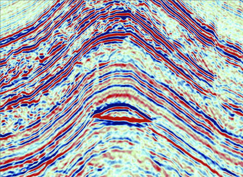
Direct Hydrocarbon Indicators (DHIs) are anomalous seismic amplitudes driven by the presence of hydrocarbons in rock. In the best case they create structurally conformant “flat spots” in seismic data, which provide very strong evidence for hydrocarbon presence.
I won’t go into details about the underlying physics in this post, focussing more on how to handle them probabilistically. DHIs are not perfect indicators, and how to integrate their presence or absence in oil and gas exploration risking is often the subject of debate.
A recent discussion about a paper1 had me realise I have many thoughts on this topic, so I decided to write them down here.
The first place I go with this is the analogy to medical testing. A DHI can be seen as a kind of “test” that provides imperfect information about some outcome (the presence or absence of hydrocarbons, in the simplest binary case). This framing falls into the realm of confusion matrices.
Using confusion matrices to quantify how probabilities are updated in the presence or absence of DHIs is very useful, and also yields some unintuitive results that I think are often neglected during the lively arguments that often spring up around them.
First, some quick background on confusion matrices and Bayes, before going back to the specific case of DHIs:
Confusion matrices
Confusion matrices, in their simplest form, separate observations into four categories, which map well onto a medical testing context:
| Disease present (\(H\)) | Disease absent (\(\neg H\)) | |
|---|---|---|
| Test positive (+) | True Positive (TP) | False Positive (FP) |
| Test negative (-) | False Negative (FN) | True Negative (TN) |
They can be generalized to multi-outcome classification, as well, which I’ll get to later in this post.
A dataset that classifies observations into these buckets can be used to do a lot of helpful inference about the strength of evidence that a test provides towards some hypothesis (H).
In the case of oil and gas prospecting in the presence of DHIs, the buckets become:
| Hydrocarbons present (\(H\)) | Hydrocarbons absent (\(\neg H\)) | |
|---|---|---|
| DHI observed (+) | True Positive (TP) | False Positive (FP) |
| No DHI observed (-) | False Negative (FN) | True Negative (TN) |
The most important calculations, that will get us to bayesian updating are as follows:
Sensitivity
\[ \begin{aligned} \text{Sensitivity} &= P(+ \mid H) \\[10pt] &= \frac{TP}{TP + FN} \end{aligned} \]
Sensitivity is the true-positive rate: how often the test is positive when the hypothesis \(H\) is true.
Specificity
\[ \begin{aligned} \text{Specificity} &= P(- \mid \neg H) \\[10pt] &= \frac{TN}{TN + FP} \end{aligned} \]
Specificity is the true-negative rate: how often the test is negative when the hypothesis \(H\) is false.
Likelihood Ratios
\[ \begin{aligned} \mathrm{LR}^{+} &= \frac{P(+ \mid H)}{P(+ \mid \neg H)} \\[10pt] &= \frac{\text{Sensitivity}}{1 - \text{Specificity}} \end{aligned} \]
Positive likelihood ratio tells how strongly a positive test result shifts evidence toward \(H\).
\[ \begin{aligned} \mathrm{LR}^{-} &= \frac{P(- \mid H)}{P(- \mid \neg H)} \\[10pt] &= \frac{1 - \text{Sensitivity}}{\text{Specificity}} \end{aligned} \]
Negative likelihood ratio tells how strongly a negative test result shifts evidence away from \(H\).
Notice that we have both positive and negative likelihood ratios, they are not the same. This will become important.
Using likelihood ratios with Bayes
A source of confusion and frustration: the probability we care about is not
\(P(+ \mid H)\) – The probability of observing the test result, given our hypothesis is true,
but actually
\(P(H \mid +)\) – The probability our hypothesis is true, given the test result.
There is at least one book written on this topic and it may leave you convinced that this difference is why statistics, science and basically everything else, suck. I recommend it!
Lucky for us it is an easy fix, in this case. We can calculate that probability using Bayes theorem:
\[ P(H \mid +) = \frac{P(+ \mid H)P(H)}{P(+)} \]
\(P(H)\) is the prior probability for the hypothesis (how likely we think it is before looking at evidence), which we can argue over, but is at least intuitive to think about. In the oil and gas context, this is the geological chance of success (COS), importantly without regard for the DHI.
\(P(+)\) is the probability… of the evidence. Which is annoying to calculate in the best case, and in worse (and common) cases, actually impossible.
Fortunately, we can rearrange things in this context to make the calculation convenient.
Using odds to make Bayes easier
If I had any advice for making Bayes less confusing, it would be to think (and calculate) in terms of odds, not probabilities.
Converting to odds is simply done:
\[ \text{Prior odds} = \frac{P(H)}{1 - P(H)} \]
Then, the math works out that the posterior odds are calculated as the prior odds multiplied by the likelihood ratio, which we calculated using the confusion matrix:
\[ \text{Posterior odds} = \text{Prior odds} \times \mathrm{LR}^{+} \]
Converting back from odds to probability gets us to the probability we care about:
\[ P(H \mid +) = \frac{\text{Posterior odds}}{1 + \text{Posterior odds}} \]
If you are so inclined, log-transforming odds turns the multiplication into addition, which is easier to work with:
\[ \log\!\left(\text{Posterior odds}\right) = \log\!\left(\text{Prior odds}\right) + \log\!\left(\mathrm{LR}^{+}\right) \]
This might seem like a lot of faff, but once you get your head around it Bayes becomes a lot more intuitive, and rough mental calculations become possible.
Neglecting the negative case
Something that struck me while reading the paper is that the data used is described as a global database of previous wildcat wells and their postdrill results. This includes DHI and non DHI supported wildcats. That is great, and it is no doubt one of the largest datasets of its kind.
The issue is that the paper then focusses on the DHI supported data only, using a 185 row subset of the dataset in a supervised machine learning DHI rating system.
But all those wildcats drilled without DHI support are an essential part of the dataset!
In fact, a Bayesian update can’t be calculated without them, due to the absence of the False Negative and True Negative quadrants in the confusion matrix. These are needed to compute Sensitivity and Specificity, which are in turn needed for computing Likelihood Ratios.
This has some consequences that I’ll go into more in the following sections.
Example dataset
Imagine we’ve catalogued all prospects over a region into a simple dataset, noting when hydrocarbons are encountered and when a DHI is present or absent. For now, we’re ignoring other covariates like depth, data quality etc:
Note that, despite DHIs being the thing we care about when tabulating this data, we are tracking all the times a DHI was absent, as well.
Using these counts directly, we can compute sensitivity, specificity, and likelihood ratios:
\[ \begin{aligned} \text{Sensitivity} &= \frac{TP}{TP + FN} \\ &= \frac{25}{40} \\[8px] &= 0.6250 \end{aligned} \]
\[ \begin{aligned} \text{Specificity} &= \frac{TN}{TN + FP} \\ &= \frac{30}{32} \\[8px] &= 0.9375 \end{aligned} \]
\[ \begin{aligned} \mathrm{LR}^{+} &= \frac{\text{Sensitivity}}{1 - \text{Specificity}} \\ &= \frac{0.6250}{1 - 0.9375} \\[8px] &= 10.0000 \end{aligned} \]
\[ \begin{aligned} \mathrm{LR}^{-} &= \frac{1 - \text{Sensitivity}}{\text{Specificity}} \\ &= \frac{1 - 0.6250}{0.9375} \\[8px] &= 0.4000 \end{aligned} \]
Now we can plug whatever prior probability we want into Bayes theorem along with the likelihood ratios and calculate posterior probabilities.
Probability updates
Probability updates are often visualized with a prior vs posterior crossplot, where a diagonal line indicates no change, and posterior probabilities are plotted as a line bowing out from it. This makes visual the update that occurs at any prior probability, given the presence or absence of the DHI:
This creates an intuitive sense that stronger evidence (a high likelihood ratio) causes more flex in the probability, either up or down.
A DHI gives the chance of success a boost (green line), whereas the absence of a DHI hurts it (orange line).
For example, if our geological COS for a prospect is at 50%, the update a DHI provides us, given the likelihood ratios derived from the confusion matrix, are as shown:
| Prior COS | Posterior COS | |
|---|---|---|
| Case | ||
| DHI observed | 0.5 | 0.909091 |
| No DHI observed | 0.5 | 0.285714 |
There are a few things to note here.
For one thing, the updates are not linear. Postively updating from 0.1 appears more dramatic than updating from 0.9. And in the probability domain, this is true, but in the log-odds domain these lines are all parallel, changing likelihood ratios just shifts them up and down on the posterior log odds axis. It is useful to internalize this because it leads you to realise there’s nothing magical happening with those curves, the same information is being incorporated into the posterior – where you start from (your prior) isn’t changing the underlying mechanics.
The other important thing is that positive and negative updates are not symmetrical. The supporting evidence a DHI provides is not the same as evidence against if the DHI is absent.
This is unintuitive (if you ask me, at least) and it makes ruling out prospects with no DHI support a potentially irrational thing to do. If DHI specificity is not very high (as in this example), it indicates DHI absence is not a deal breaker for a prospect, even if DHI presence would make it a slam dunk!
So if all the geological elements are very high confidence, and you’ve agreed to a COS of 0.85, don’t let a geophysicist crash the party without providing real justification.
If that geophysicist draws a version of the above plot patiently explaining why you, the simple minded geologist, aren’t getting it, ask them why the plot is symmetrical.
They might get smug and say something like:
Well logically, the confidence the DHI gives us, and the confidence it takes away, are the same thing
but they’ll be wrong.
Most of these “probability update” crossplots I’ve seen on this topic (including the one in the paper I mentioned) are symmetrical, so I think this point is often missed.
This is a downstream consequence of neglecting the non DHI supported data, as this takes probability out of its full context, leading to people using precise numbers to be precisely wrong.
Better handling uncertainty
Confusion matrices happen to fit nicely into something called a Dirichlet-multinomial conjugate model. I’ve written briefly about the nice properties of this distribution here.
Basically, since each quadrant of the confusion matrix is exclusive and exhaustive (all observations are one of TP, TN, FP, FN), those counts can be used to parametrize a distribution over their respective frequencies, which amounts to a set of probabilities that form a unit simplex (sum to 1.0).
The \(\alpha\) vector that parameterizes the Dirichlet distribution is simply the count in each bin of the confusion matrix, with a prior (for example, a vector of 1.0 for uniform priors). This is very convenient, as new data can just be encoded as updating counts, yielding an updated distribution.
Since data is very scarce in this context (drilling wells is expensive), this is a nice property to take advantage of. It means that quantities like the Sensitivity and Specificity, as well as the positive and negative Likelihood Ratios, are estimated as probability distributions, rather than deterministic quantities. The uncertainty of the estimates is a function of the number of observations in the dataset. Many observations means less uncertainty.
To see what the Dirichlet model is doing directly, we can look at the sampled probability for each confusion-matrix category:
The frequency that each category is present in the dataset are plotted as vertical lines, but there are a range of plausible values surrounding them that could equally have given rise to our dataset.
The resulting distributions for sensitivity and specificity (calculated by plugging in the array of probability values, instead of the single calculated values) look like this:
And finally, likelhood ratios (and the associated prior to posterior update) are represented as distributions, which lets us show a range of plausible probability updates given our data:
Now, not only is the asymmetry of updates evident, but the asymmetry in the uncertainty about them is too. The way these differences come about is a bit of a headache, but is all a function of the prior, the number of datapoints we have in each category, and the equations shown in the earlier section.
Example Prior = 0.5
It may seem odd to arrive at a range of possible posterior probabilities when we’re accustomed to using single numbers. But, consider that we don’t know how strong the DHI is as an indicator, we have been tricked before, and we don’t have much data. That means there is a fair amount of uncertainty about what our posterior probability could be when considering the DHI. It is possible to propagate this uncertainty into volumetric models, but in practice we usually just run with an agreed upon single value.
Whether the full distribution is used or not, the point is it is unwise to get hung up on a single correct value, when there is a lot of uncertainty left on the table.
Not all DHIs are the same
Fancy statistics aside, something this approach still leaves out is that not all DHIs are equal in terms of the information they provide. A clear flat spot that strongly conforms to structure, in a lithology and depth window that we physically expect should show such a contrast, is very convincing evidence of hydrocarbon presence. In contrast, an amorphous amplitude anomaly that we think may correspond to a sand body in poorly processed seismic data, is much less convincing.
Some additional variables that should be included are:
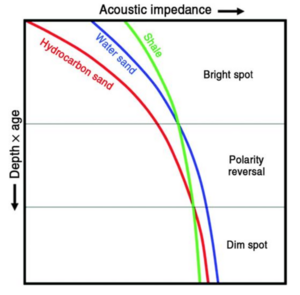
Depth: it is expected that acoustic impedance contrasts, and the respective effects of pore fluid will change with depth, leading to different DHI characteristics
Structural Conformance: DHI flat spots that conform well to structure are expected to be more reliable, so an ordinal index tracking this should be included in the model
Signal Strength: The strength of the amplitude anomaly should increase confidence in its validity (vs random noise)
Data Quality: Lower quality, noisier seismic data yields less confidence than anomalies observed on high quality datasets
The paper that led to me writing this has a nice risk-matrix showing their schema for rating DHI “discernability”, which considers both the expectation of a DHI response (given the geological and geophysical context) and the confidence in the data.
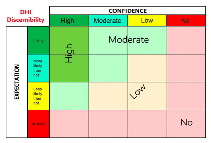
Their discernability metric appears to be equivalent to the likelihood ratio applied here, but is estimated using the above matrix.
With a rich dataset, I would model DHI as a diagnostic signal conditional on hydrocarbon state and prospect context, then convert that into context-dependent likelihood ratios for Bayesian updating. This moves out of classification and into logistic regression.
\[ Y_i \sim \operatorname{Bernoulli}(\pi_i) \]
\[ \operatorname{logit}\!\big(P(Y_i=1 \mid H_i=h,\mathbf{x}_i)\big) = \alpha_h + f_h(d_i) + \mathbf{x}_i^\top \boldsymbol{\gamma}_h \]
Where:
- \(i\) indexes prospect reservoir intersections
- \(Y_i\) is the observed DHI indicator (\(1=\mathrm{DHI\ present},\;0=\mathrm{DHI\ absent}\))
- \(H_i\) is hydrocarbon state (\(1=\mathrm{HC},\;0=\mathrm{no\ HC}\))
- \(\pi_i = P(Y_i=1 \mid H_i,\mathbf{x}_i)\)
- \(d_i\) is depth
- \(\mathbf{x}_i\) are additional predictors (for example structural conformance, signal strength, data quality)
- \(\alpha_h\), \(f_h(\cdot)\), and \(\boldsymbol{\gamma}_h\) are hydrocarbon-state-specific intercepts/effects
This gives two conditional DHI-response models: one for hydrocarbon presence and one for hydrocarbon absence. From these, context dependent likelihood ratios are calculated as:
\[ \operatorname{LR}^{+}(\mathbf{x}) = \frac{P(Y=1 \mid H=1,\mathbf{x})}{P(Y=1 \mid H=0,\mathbf{x})} \]
\[ \operatorname{LR}^{-}(\mathbf{x}) = \frac{P(Y=0 \mid H=1,\mathbf{x})}{P(Y=0 \mid H=0,\mathbf{x})} \]
These context-dependent likelihood ratios can then be used with prior odds to obtain posterior \(P(H=1\mid Y,\mathbf{x})\) for new prospects.
Think of the update crossplot above bowing in and out depending on the depth, data quality, structural conformance etc of the prospect in question. That is essentially what the model would be doing.
Incorporating the physics more directly in a model is something I’m interested in playing with as well, though I’ve not done it before. Incorporating rock physics data means the acoustic impedance vs depth trend could be estimated, which along with fluid substitution would mean DHI amplitude anomalies could be simulated physically for different pore fluids and reservoirs, providing posterior probabilities over each scenario given what is observed at the target interval.
Is success and failure really enough?
A final extension of this is based on a fairly simple point:
Why are we talking about “success” and “failure” as if those are the canonical outcomes of drilling a prospect?
In the context of DHIs and oil and gas prospecting, a “failure” could mean several different things:
- There is gas at the anomaly, and we wanted oil
- There is gas at the anomaly, but it is at residual saturation and non economic
- The reservoir is water saturated
- There is no reservoir at the anomaly
And a “success” depends on what we care about… but DHI’s don’t care about that.
Confusion matrices, as I mentioned earlier, can be extended to multiple outcome states, where the “test” of the DHI has an associated likelihood ratio for each of them.
For this example I’ll use the following states, though more or less could be included as long as they represent an exhaustive set:
- Oil
- Gas
- Fizz (low saturation gas)
- Water
- Shale (no reservoir)
A simple toy dataset for these expanded states might look like this:
| DHI observed | No DHI observed | |
|---|---|---|
| State | ||
| Oil | 25 | 8 |
| Gas | 18 | 4 |
| Fizz | 10 | 12 |
| Water | 4 | 25 |
| Shale | 1 | 30 |
Using a prior probability over each state, we can sample the posterior state probabilities given a DHI and visualize the uncertainty for each:
| Prior Probability | |
|---|---|
| State | |
| Oil | 0.2500 |
| Gas | 0.5000 |
| Fizz | 0.1250 |
| Water | 0.0625 |
| Shale | 0.0625 |
And we can do the same update for the absence of a DHI:
This shifts from thinking in terms of “will the prospect succeed or fail” to a more granular “what do we expect to find when we drill the prospect” set of scenarios. Fizz, water and shale can be summed to a single “Failure” scenario, but the oil and gas scenarios certainly benefit from separate scenario based economic analyses.
The challenge with this kind of approach is calibration – the more categories are split, the more sparse our datasets are. There are ways of mitigating this in bayesian statistics via hierarchical models/partial pooling, but it is still a challenge.
Closing thoughts
Absent the data, it can still be useful to have these frameworks in mind, as more subjective inputs can still be put through a probabilistically rigorous process, meaning that at the very least, the outputs are logical consequences of the inputs.
And maybe this all seems over the top. “Don’t overscience it” is a refrain I’ve heard plenty of times in my career. I’m sympathetic to not tricking ourselves into being precisely wrong with overly complicated theories. That is part of why bayesian methods appeal to me so much – uncertainty is a first class citizen.
But we are usually talking about hundreds of millions of dollar decisions in this context, so maybe sciencing the hell out of it is a good investment?
Thanks for reading.
Footnotes
Monigle, P. W., Hedayati, T. S., and Goulding, F. J., 2025, Integrated and improved direct hydrocarbon indicators: A step forward in petroleum risk discrimination: AAPG Bulletin, 109(5), 617-636, https://doi.org/10.1306/04042524030.↩︎