import matplotlib.pyplot as plt
import numpy as np
import pandas as pd

import drisk as drCorrelated Discrete Outcomes
Bernoulli race wins with a Gaussian copula
Motivation
A trainer is planning a short campaign for one horse across several races. Each race has its own win probability because the field, distance, and track conditions differ. If we sample each race independently, we assume the horse’s result in one race tells us nothing about its likely result in the others.
That is often too strong. A horse may have an unobserved underlying form, soundness, or capacity that persists across the campaign. If the horse is better than expected, several wins become more likely; if it is off-form, several losses become more likely. The races are not perfectly locked together, but they are also not independent.
A Gaussian copula with Bernoulli marginals is a compact way to represent this: keep the elicited probability for each race, then add positive dependence between the binary win outcomes.
Elicit race-level win probabilities
Each Bernoulli distribution represents the event “our horse wins this race”.
race_inputs = [
    ("Sprint prep", 0.18),
    ("Allowance", 0.22),
    ("Turf mile", 0.15),
    ("Local stakes", 0.28),
    ("Dirt route", 0.12),
    ("Handicap", 0.20),
    ("Feature stakes", 0.25),
    ("Final sprint", 0.16),
]

race_wins = [
    dr.Bernoulli.elicit(p, name=name)
    for name, p in race_inputs
]

pd.DataFrame(race_inputs, columns=["race", "p_win"])| race | p_win | |
|---|---|---|
| 0 | Sprint prep | 0.18 |
| 1 | Allowance | 0.22 |
| 2 | Turf mile | 0.15 |
| 3 | Local stakes | 0.28 |
| 4 | Dirt route | 0.12 |
| 5 | Handicap | 0.20 |
| 6 | Feature stakes | 0.25 |
| 7 | Final sprint | 0.16 |
Independent campaign simulation
First simulate the campaign as if the eight race outcomes were independent.
size = 50_000
rng = np.random.default_rng(42)

independent_race_samples = np.vstack([
    race.sample(size=size, seed=rng)
    for race in race_wins
])
independent_total_wins = independent_race_samples.sum(axis=0)

independent_total_wins.mean()np.float64(1.55184)The expected number of wins is just the sum of the race probabilities, but the shape of the total-win distribution depends strongly on the independence assumption.
Compare campaign win counts
Positive dependence moves probability mass toward more clustered outcomes: more campaigns with no wins, and more campaigns with several wins. The average number of wins is almost unchanged because the individual race probabilities are unchanged.
def win_count_distribution(samples: np.ndarray, n: int) -> np.ndarray:
    return np.bincount(samples.astype(int), minlength=n + 1)[: n + 1] / samples.size

comparison = pd.DataFrame(
    {
        "independent": win_count_distribution(independent_total_wins, n_races),
        "correlated": win_count_distribution(correlated_total_wins, n_races),
    },
    index=pd.Index(range(n_races + 1), name="total wins"),
)

comparison| independent | correlated | |
|---|---|---|
| total wins | ||
| 0 | 0.17624 | 0.60694 |
| 1 | 0.34132 | 0.09762 |
| 2 | 0.29536 | 0.05814 |
| 3 | 0.13768 | 0.04372 |
| 4 | 0.04110 | 0.03670 |
| 5 | 0.00748 | 0.03264 |
| 6 | 0.00078 | 0.03270 |
| 7 | 0.00004 | 0.03400 |
| 8 | 0.00000 | 0.05754 |
summary = pd.DataFrame(
    {
        "independent": {
            "mean wins": independent_total_wins.mean(),
            "p(no wins)": np.mean(independent_total_wins == 0),
            "p(3+ wins)": np.mean(independent_total_wins >= 3),
        },
        "correlated": {
            "mean wins": correlated_total_wins.mean(),
            "p(no wins)": np.mean(correlated_total_wins == 0),
            "p(3+ wins)": np.mean(correlated_total_wins >= 3),
        },
    }
).T

summary| mean wins | p(no wins) | p(3+ wins) | |
|---|---|---|---|
| independent | 1.55184 | 0.17624 | 0.18708 |
| correlated | 1.54958 | 0.60694 | 0.23730 |
fig, ax = plt.subplots(figsize=(8, 4.5))
x = np.arange(n_races + 1)
width = 0.38

ax.bar(
    x - width / 2,
    comparison["independent"],
    width=width,
    label="Independent races",
    color="#4C78A8",
)
ax.bar(
    x + width / 2,
    comparison["correlated"],
    width=width,
    label="Correlated form",
    color="#F58518",
)

ax.set_title("Campaign total wins")
ax.set_xlabel("Total wins across campaign")
ax.set_ylabel("Probability")
ax.set_xticks(x)
ax.legend()
fig.tight_layout()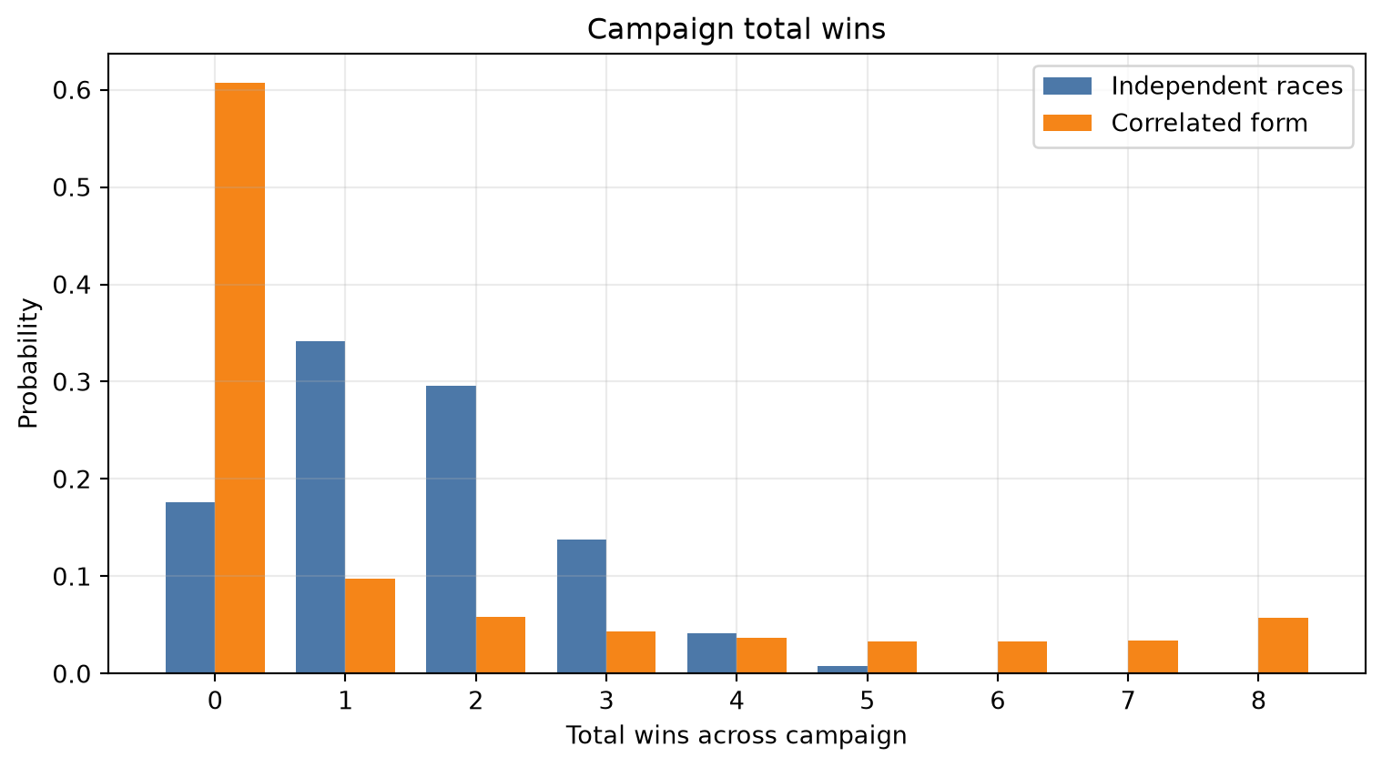
Using the same copula in a composed model
The direct copula samples above are useful when you want to inspect the joint binary outcomes. The same copula can also be attached to an arithmetic MCModel. Here the model is simply the sum of race wins.
campaign_wins = race_wins[0]
for race in race_wins[1:]:
    campaign_wins = campaign_wins + race
campaign_wins.name = "Campaign wins"

campaign_wins.add_copula(form_copula)
campaign_wins.summary(size=size, seed=42, threshold=2, precision=3)| mean | p(> 2) | p99 | p90 | p75 | p50 | p25 | p10 | p1 | |
|---|---|---|---|---|---|---|---|---|---|
| metric | |||||||||
| Campaign wins | 1.55 | 0.237 | 0.0 | 0.0 | 0.0 | 0.0 | 2.0 | 6.0 | 8.0 |
The important point is that there is no separate outcome-specific copula API here. Correlated binary outcomes are just Bernoulli marginal distributions sampled through the same GaussianCopula machinery used for continuous distributions.