Composing Discrete and Continuous Distributions

Annual equipment-failure cost and downtime

Motivation

A field-operations team maintains a small fleet of pumps. They need a rough annual maintenance plan that accounts for two kinds of uncertainty:

how many pump failures occur in a year, and
the average cost and downtime per failure.

A Poisson distribution is a natural model for the count of failures in a fixed period. Repair cost and downtime are positive, right-skewed quantities. We will use a lognormal distribution for average repair cost and a PERT distribution for average downtime. In this example, these distributions represent the average per-failure outcome for the year, which makes the annual model easy to write as ordinary arithmetic:

annual outcome = number of failures * average outcome per failure

import matplotlib.pyplot as plt

import drisk as dr

Elicit the inputs

The reliability engineer expects about five pump failures per year across the fleet.

failures = dr.Poisson.elicit(
    lam=5.0,
    name="Pump failures per year",
)

For planning, the team estimates that the average repair cost per failure will usually fall between $3,000 and $12,000. For average downtime, the engineer provides a three-point estimate: optimistic, most likely, and pessimistic hours per failure.

avg_repair_cost = dr.LogNormal.elicit(
    lower=3_000,
    upper=12_000,
    confidence=0.8,
    name="Average repair cost per failure",
)

avg_downtime_hours = dr.PERT.elicit(
    min=4,
    mode=12,
    max=36,
    name="Average downtime hours per failure",
)

The elicited shapes are easy to check before composing the model.

fig, axes = plt.subplots(1, 3, figsize=(12, 3.5))
failures.plot(ax=axes[0], color="#4C78A8")
avg_repair_cost.plot(ax=axes[1], color="#F58518")
avg_downtime_hours.plot(ax=axes[2], color="#54A24B")
fig.tight_layout()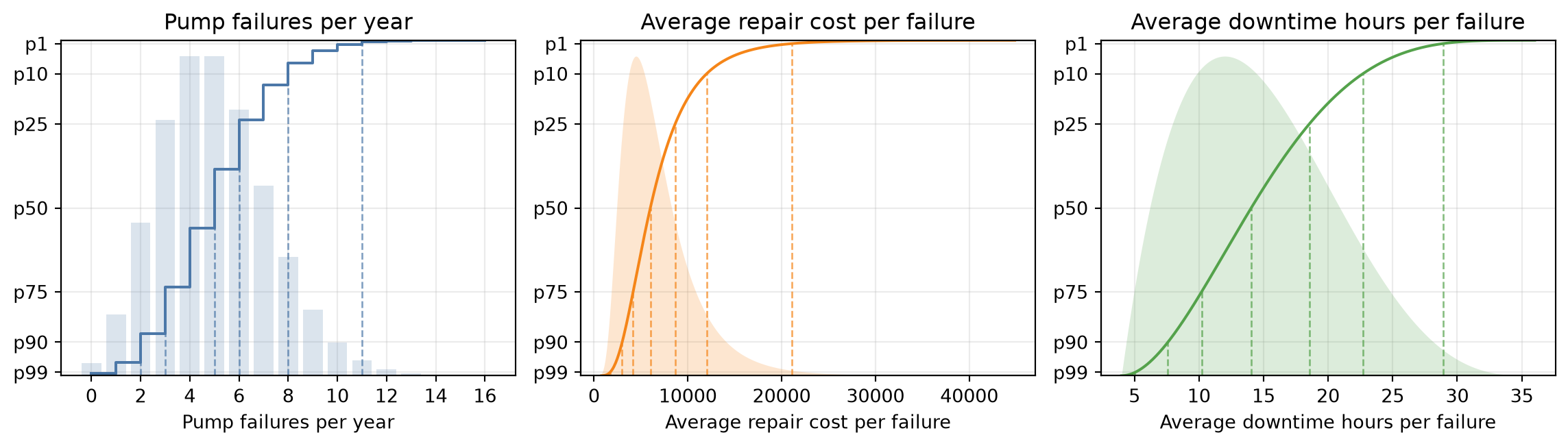

Compose annual outcomes

Because drisk distributions support arithmetic, the annual outcomes read like the underlying planning logic.

annual_repair_cost = failures * avg_repair_cost
annual_repair_cost.name = "Annual repair cost"

annual_downtime_hours = failures * avg_downtime_hours
annual_downtime_hours.name = "Annual downtime hours"

type(annual_repair_cost).__name__

'MCModel'

The count distribution is discrete and the average-outcome distributions are continuous, but the composed results are both sampleable MCModel expressions.

Simulate the annual plan

repair_summary = annual_repair_cost.summary(
    size=50_000,
    seed=42,
    threshold=50_000,
)
downtime_summary = annual_downtime_hours.summary(
    size=50_000,
    seed=42,
    threshold=120,
)

repair_summary

	mean	p(> 50000)	p99	p90	p75	p50	p25	p10	p1
metric
Annual repair cost	34747.86	0.2	2782.42	10081.42	16736.91	27734.82	44909.51	67337.39	133181.73

downtime_summary

	mean	p(> 120)	p99	p90	p75	p50	p25	p10	p1
metric
Annual downtime hours	73.4	0.14	7.22	24.78	40.22	64.14	96.75	134.96	215.47

cost_values = repair_summary.loc["Annual repair cost"]
downtime_values = downtime_summary.loc["Annual downtime hours"]

print(f"Mean annual repair cost: ${cost_values['mean']:,.0f}")
print(
    "P10 / P50 / P90 annual repair cost: "
    f"${cost_values['p10']:,.0f} / ${cost_values['p50']:,.0f} / ${cost_values['p90']:,.0f}"
)
print(f"Probability annual repair cost exceeds $50k: {cost_values['p(> 50000)']:.1%}")
print()
print(f"Mean annual downtime: {downtime_values['mean']:,.0f} hours")
print(
    "P10 / P50 / P90 annual downtime: "
    f"{downtime_values['p10']:,.0f} / {downtime_values['p50']:,.0f} / {downtime_values['p90']:,.0f} hours"
)
print(f"Probability annual downtime exceeds 120 hours: {downtime_values['p(> 120)']:.1%}")

Mean annual repair cost: $34,748
P10 / P50 / P90 annual repair cost: $67,337 / $27,735 / $10,081
Probability annual repair cost exceeds $50k: 20.0%

Mean annual downtime: 73 hours
P10 / P50 / P90 annual downtime: 135 / 64 / 25 hours
Probability annual downtime exceeds 120 hours: 14.0%

Present the result

fig, axes = plt.subplots(1, 2, figsize=(12, 4.5))

annual_repair_cost.plot(
    ax=axes[0],
    size=50_000,
    seed=42,
    color="#F58518",
)
axes[0].axvline(50_000, color="black", linestyle="--", linewidth=1, label="$50k budget")
axes[0].legend()

annual_downtime_hours.plot(
    ax=axes[1],
    size=50_000,
    seed=42,
    color="#54A24B",
)
axes[1].axvline(120, color="black", linestyle="--", linewidth=1, label="120 hours")
axes[1].legend()

fig.tight_layout()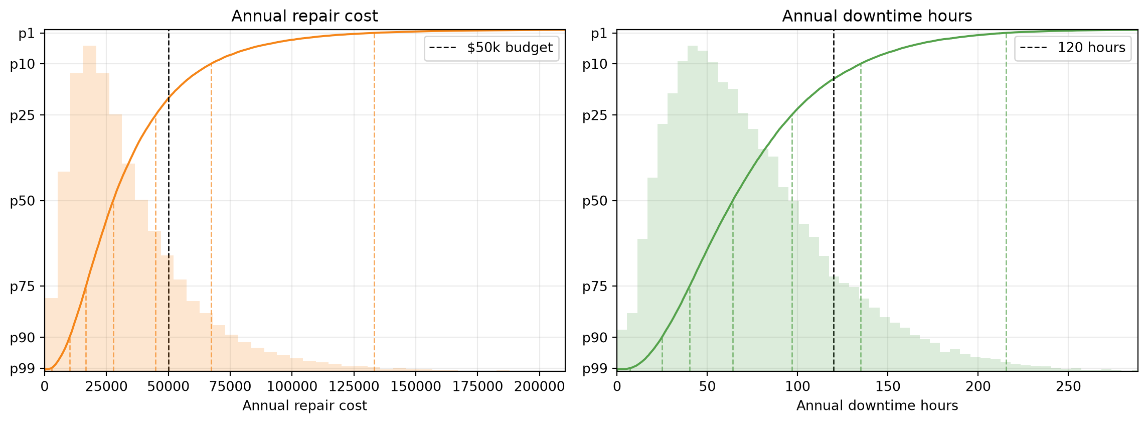

What this composition assumes

This compact model samples one average repair cost and one average downtime for each simulated year. That is appropriate when the elicited lognormal distributions represent uncertainty about the annual average outcome per failure, not the outcome of every individual failure.

If the question changes to modeling each individual repair, the same ingredients can be used in a richer simulation: sample the number of failures, then sample and sum one cost or downtime value for each failure. The arithmetic composition shown here is the simpler planning model.