import matplotlib.pyplot as plt
import numpy as np
import pandas as pd

import drisk as drCorrelated Sampling with Copulas
Adding dependence to the product launch model
Motivation
The composition example treated each uncertain input as independent. In many real models, inputs move together: a larger addressable market might also imply higher fixed launch costs, and price and unit cost may be positively related.
drisk lets you keep the same arithmetic expression and then attach correlated sampling to the resulting MCModel. The convenience method .correlate(...) builds a Gaussian copula over the model’s distribution inputs.
Build the same model
We use the same elicited inputs and profit expression as the Monte Carlo composition example.
market_size = dr.PERT.elicit(
    min=20_000,
    mode=50_000,
    max=100_000,
    name="Addressable market size",
)

conversion = dr.LogitNormal.elicit(
    lower=0.02,
    upper=0.08,
    confidence=0.8,
    name="Conversion rate",
)

price = dr.LogNormal.elicit(
    lower=40,
    upper=80,
    confidence=0.8,
    name="Average selling price",
)

unit_cost = dr.PERT.elicit(
    min=12,
    mode=18,
    max=30,
    name="Unit cost",
)

fixed_cost = dr.PERT.elicit(
    min=100_000,
    mode=150_000,
    max=250_000,
    name="Fixed launch cost",
)

profit = market_size * conversion * (price - unit_cost) - fixed_cost
Before adding correlations, the model’s distribution leaves are sampled independently.
independent_samples = profit.sample(size=50_000, seed=42)
independent_summary = profit.summary(threshold=0)
independent_summary| mean | p(> 0) | p99 | p90 | p75 | p50 | p25 | p10 | p1 | |
|---|---|---|---|---|---|---|---|---|---|
| metric | |||||||||
| value | -59958.86 | 0.17 | -183166.16 | -142182.21 | -114149.73 | -77754.02 | -27099.81 | 40256.46 | 244085.91 |
Check distribution order
A full correlation matrix is interpreted in the order returned by .distributions(): first appearance in the arithmetic expression.
[dist.name for dist in profit.distributions()]['Addressable market size',
'Conversion rate',
'Average selling price',
'Unit cost',
'Fixed launch cost']For this expression, the order is:
- addressable market size,
- conversion rate,
- average selling price,
- unit cost, and
- fixed launch cost.
Apply a correlation matrix
Pass a full correlation matrix to .correlate(...). Under the hood, drisk creates a GaussianCopula for these marginal distributions and attaches it to the MCModel, so .sample(), .summary(), and .plot() all use correlated draws from that point on.
correlation_matrix = [
    [1.00, 0.45, 0.15, 0.20, 0.35],
    [0.45, 1.00, 0.20, 0.10, 0.15],
    [0.15, 0.20, 1.00, 0.60, 0.05],
    [0.20, 0.10, 0.60, 1.00, 0.10],
    [0.35, 0.15, 0.05, 0.10, 1.00],
]

profit.correlate(correlation_matrix)
MCModel(op=<MCOperation.SUBTRACT: 'subtract'>, operands=(MCModel(op=<MCOperation.MULTIPLY: 'multiply'>, operands=(MCModel(op=<MCOperation.MULTIPLY: 'multiply'>, operands=(PERT(dist_type='pert', name='Addressable market size', elicitation_params={'min': 20000, 'mode': 50000, 'max': 100000, 'concentration': 4.0}, params={'min': 20000.0, 'max': 100000.0, 'alpha': 2.5, 'beta': 3.5, 'mode': 50000.0, 'concentration': 4.0}), LogitNormal(dist_type='logitnormal', name='Conversion rate', elicitation_params={'lower': 0.02, 'upper': 0.08, 'confidence': 0.8}, params={'mu': -3.1670836667399156, 'sigma': 0.5655149982690953})), name=None, copula=None), MCModel(op=<MCOperation.SUBTRACT: 'subtract'>, operands=(LogNormal(dist_type='lognormal', name='Average selling price', elicitation_params={'lower': 40, 'upper': 80, 'confidence': 0.8}, params={'mu': 4.0354530443939085, 'sigma': 0.27043280941465253}), PERT(dist_type='pert', name='Unit cost', elicitation_params={'min': 12, 'mode': 18, 'max': 30, 'concentration': 4.0}, params={'min': 12.0, 'max': 30.0, 'alpha': 2.333333333333333, 'beta': 3.6666666666666665, 'mode': 18.0, 'concentration': 4.0})), name=None, copula=None)), name=None, copula=None), PERT(dist_type='pert', name='Fixed launch cost', elicitation_params={'min': 100000, 'mode': 150000, 'max': 250000, 'concentration': 4.0}, params={'min': 100000.0, 'max': 250000.0, 'alpha': 2.333333333333333, 'beta': 3.6666666666666665, 'mode': 150000.0, 'concentration': 4.0})), name=None, copula=GaussianCopula(distributions=(PERT(dist_type='pert', name='Addressable market size', elicitation_params={'min': 20000, 'mode': 50000, 'max': 100000, 'concentration': 4.0}, params={'min': 20000.0, 'max': 100000.0, 'alpha': 2.5, 'beta': 3.5, 'mode': 50000.0, 'concentration': 4.0}), LogitNormal(dist_type='logitnormal', name='Conversion rate', elicitation_params={'lower': 0.02, 'upper': 0.08, 'confidence': 0.8}, params={'mu': -3.1670836667399156, 'sigma': 0.5655149982690953}), LogNormal(dist_type='lognormal', name='Average selling price', elicitation_params={'lower': 40, 'upper': 80, 'confidence': 0.8}, params={'mu': 4.0354530443939085, 'sigma': 0.27043280941465253}), PERT(dist_type='pert', name='Unit cost', elicitation_params={'min': 12, 'mode': 18, 'max': 30, 'concentration': 4.0}, params={'min': 12.0, 'max': 30.0, 'alpha': 2.333333333333333, 'beta': 3.6666666666666665, 'mode': 18.0, 'concentration': 4.0}), PERT(dist_type='pert', name='Fixed launch cost', elicitation_params={'min': 100000, 'mode': 150000, 'max': 250000, 'concentration': 4.0}, params={'min': 100000.0, 'max': 250000.0, 'alpha': 2.333333333333333, 'beta': 3.6666666666666665, 'mode': 150000.0, 'concentration': 4.0})), corr_matrix=CorrelationMatrix(matrix=[[1.0, 0.45, 0.15, 0.2, 0.35], [0.45, 1.0, 0.2, 0.1, 0.15], [0.15, 0.2, 1.0, 0.6, 0.05], [0.2, 0.1, 0.6, 1.0, 0.1], [0.35, 0.15, 0.05, 0.1, 1.0]]), copula_type='gaussian'))profit.copula.corr_matrix.plot(labels=[dist.name for dist in profit.distributions()])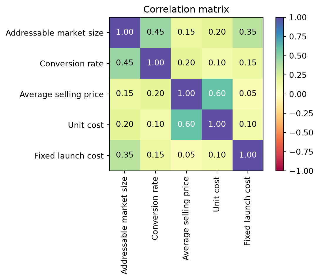
correlated_samples = profit.sample(size=50_000, seed=42)
correlated_summary = profit.summary(threshold=0)
correlated_summary| mean | p(> 0) | p99 | p90 | p75 | p50 | p25 | p10 | p1 | |
|---|---|---|---|---|---|---|---|---|---|
| metric | |||||||||
| value | -47702.68 | 0.2 | -175473.89 | -136363.4 | -110608.81 | -76220.4 | -18359.57 | 70815.24 | 368401.92 |
Compare independent and correlated runs
comparison = pd.concat(
    {
        "independent": independent_summary.loc["value"],
        "correlated": correlated_summary.loc["value"],
    },
    axis=1,
).T
comparison| mean | p(> 0) | p99 | p90 | p75 | p50 | p25 | p10 | p1 | |
|---|---|---|---|---|---|---|---|---|---|
| independent | -59958.86 | 0.17 | -183166.16 | -142182.21 | -114149.73 | -77754.02 | -27099.81 | 40256.46 | 244085.91 |
| correlated | -47702.68 | 0.20 | -175473.89 | -136363.40 | -110608.81 | -76220.40 | -18359.57 | 70815.24 | 368401.92 |
fig, ax = plt.subplots(figsize=(8, 4.5))

for label, samples, color in [
    ("Independent", independent_samples, "#4C78A8"),
    ("Correlated", correlated_samples, "#F58518"),
]:
    sorted_samples = np.sort(samples)
    ecdf = np.arange(1, sorted_samples.size + 1) / sorted_samples.size
    ax.plot(sorted_samples, ecdf, label=label, color=color)

ax.axvline(0, color="black", linestyle="--", linewidth=1, label="Break-even")
ax.set_title("Product launch profit: independent vs correlated sampling")
ax.set_xlabel("Profit")
ax.set_ylabel("cumulative probability")
ax.set_ylim(0, 1)
ax.legend()
fig.tight_layout()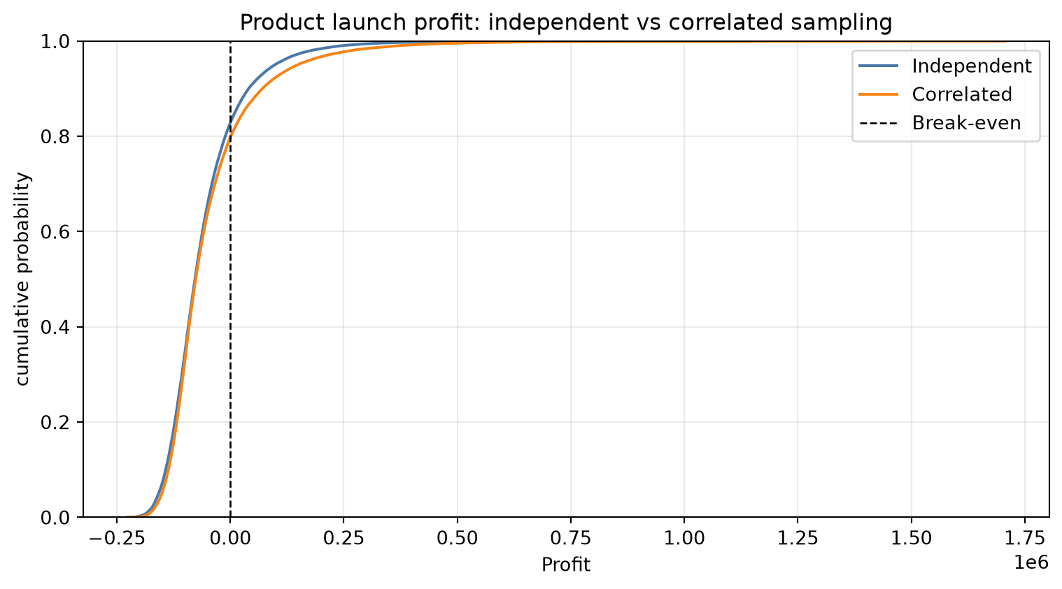
Scalar shortcut
For quick sensitivity checks, pass a single number instead of a full matrix. This applies the same off-diagonal correlation to every pair of distribution inputs.
quick_profit = market_size * conversion * (price - unit_cost) - fixed_cost
quick_profit.correlate(0.25)
quick_profit.summary(size=50_000, seed=42, threshold=0)| mean | p(> 0) | p99 | p90 | p75 | p50 | p25 | p10 | p1 | |
|---|---|---|---|---|---|---|---|---|---|
| metric | |||||||||
| value | -49128.33 | 0.2 | -169647.66 | -132581.68 | -109212.59 | -76858.46 | -21700.7 | 62446.71 | 345164.41 |
Use .add_copula(...) directly when you want to provide a specific copula object, such as a Student-t copula or a Gaussian copula constructed separately.