Composing Monte Carlo Models

A new product launch profit model

Motivation

A product team is considering a new launch. The key inputs are uncertain:

• the addressable market size,
• the share of that market that converts to customers,
• the average selling price,
• the unit cost, and
• the fixed launch cost.

With drisk, each uncertain input can be represented as an elicited distribution. The business model can then be written with ordinary Python arithmetic. Arithmetic on distribution objects returns an MCModel, a lazy Monte Carlo expression that samples each input and applies NumPy operations sample-by-sample.

import matplotlib.pyplot as plt

import drisk as dr

Elicit uncertain inputs

We use PERT distributions for expert min/mode/max estimates, a logit-normal distribution for a conversion rate bounded between 0 and 1, and a lognormal distribution for positive skew in selling price.

market_size = dr.PERT.elicit(
    min=20_000,
    mode=50_000,
    max=100_000,
    name="Addressable market size",
)

conversion = dr.LogitNormal.elicit(
    lower=0.02,
    upper=0.08,
    confidence=0.8,
    name="Conversion rate",
)

price = dr.LogNormal.elicit(
    lower=40,
    upper=80,
    confidence=0.8,
    name="Average selling price",
)

unit_cost = dr.PERT.elicit(
    min=12,
    mode=18,
    max=30,
    name="Unit cost",
)

fixed_cost = dr.PERT.elicit(
    min=100_000,
    mode=150_000,
    max=250_000,
    name="Fixed launch cost",
)

Each distribution also has a convenience .plot() method for a quick visual check of the elicited shape.

price.plot(color="limegreen")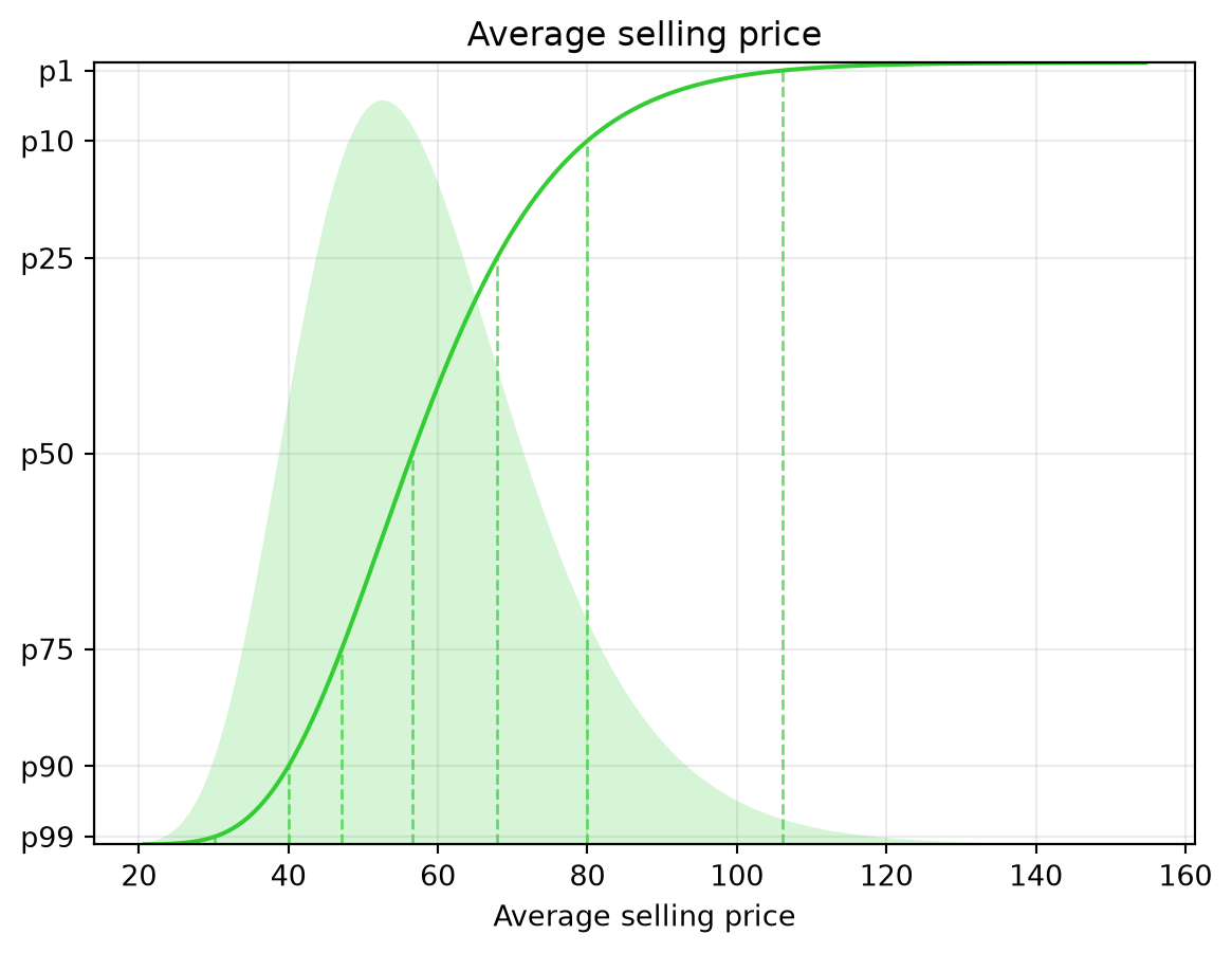

unit_cost.plot(color='salmon')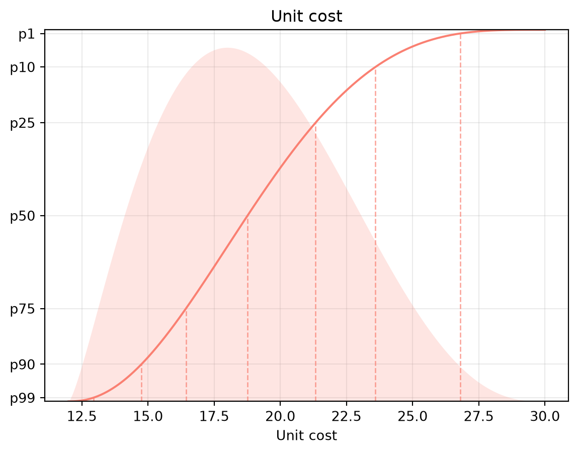

Compose the model

The profit model is just the business logic:

customers = market_size * conversion
revenue = customers * price
variable_cost = customers * unit_cost
profit = revenue - variable_cost - fixed_cost

type(profit).__name__

'MCModel'

profit is not an analytic distribution. It is an MCModel: a sampleable expression built from distributions, constants, and arithmetic operations.

Simulate outcomes

sims = profit.sample(size=50_000, seed=42)
summary = profit.summary(threshold=0)
summary

	mean	p(> 0)	p99	p90	p75	p50	p25	p10	p1
metric
value	-59958.86	0.17	-183166.16	-142182.21	-114149.73	-77754.02	-27099.81	40256.46	244085.91

Present the result

fig, ax = plt.subplots(figsize=(8, 4.5))
profit.plot(ax=ax, color="#4C78A8")
ax.set_title("Simulated product launch profit")
ax.set_xlabel("Profit")
fig.tight_layout()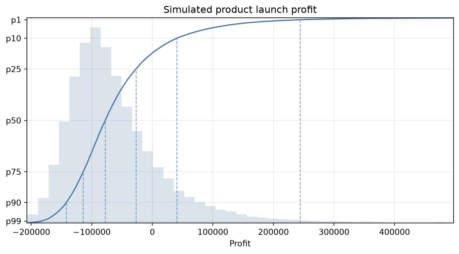

Why composition matters

The final model is readable because it mirrors the underlying decision logic:

profit = market_size * conversion * (price - unit_cost) - fixed_cost
profit.sample(size=5, seed=7)

array([-123317.17486257,  -56545.4697437 ,  -93175.65503927,
        -96029.98966468,  -99183.96846255])

That expression remains lazy until .sample(...) is called. During sampling, drisk uses a shared random number generator across the inputs and NumPy broadcasting for the sample-wise arithmetic.