Oil and Gas Prospect Evaluation

Risked oil-in-place across multiple correlated reservoirs

Motivation

A subsurface team is evaluating a prospect with several possible reservoirs. For each reservoir, the in-place volume depends on uncertain geological and fluid inputs:

porosity (phi),
water saturation (sw),
mapped area in square kilometres (area_km2),
net pay in metres (net_m), and
oil formation volume factor (bo).

Each reservoir also has a chance of geologic success. In drisk, we can express this as a composable Monte Carlo model: calculate the success-case volume, then use dr.where(...) to return zero when the reservoir fails.

import matplotlib.pyplot as plt
import numpy as np
from pydantic import BaseModel, Field

import drisk as dr

A reusable Pydantic reservoir model

Because drisk distributions and Monte Carlo expressions are Pydantic-serializable, they can be embedded in ordinary Pydantic models. Here, a Reservoir stores elicited input distributions plus a probability of success, and exposes a method that composes those inputs into a sampleable dr.MCModel.

The success-case oil in place is calculated as:

\[ \text{MMbbl} = \frac{\text{area} \cdot \text{net} \cdot \phi \cdot (1 - S_w)}{B_o} \cdot \frac{6.28981}{10^6} \]

where area is converted from square kilometres to square metres before the volume calculation. A Bernoulli distribution represents geologic success/failure, and dr.where(...) gates the success-case volume to zero when the reservoir fails.

KM2_TO_M2 = 1_000_000
M3_TO_BBL = 6.28981


class Reservoir(BaseModel):
    """Serializable reservoir inputs for a risked oil-in-place model."""

    name: str
    p_success: float = Field(ge=0, le=1)
    phi: dr.LogitNormal
    sw: dr.LogitNormal
    area_km2: dr.LogNormal
    net_m: dr.PERT
    bo: dr.LogNormal

    def success_case_oil_mmbbl(self) -> dr.MCModel:
        """Build a success-case oil-in-place model for this reservoir."""
        return (
            self.area_km2
            * KM2_TO_M2
            * self.net_m
            * self.phi
            * (1 - self.sw)
            / self.bo
            * M3_TO_BBL
            / 1e6
        )

    def oil_mmbbl(self) -> dr.MCModel:
        """Build a risked oil-in-place model for this reservoir."""
        success = dr.Bernoulli.elicit(self.p_success, name=f"{self.name} success")
        return dr.where(success, self.success_case_oil_mmbbl(), 0.0, name=self.name)

    def expected_oil_mmbbl(self) -> dr.MCModel:
        """Build an expected-value oil-in-place model for sensitivity analysis."""
        return self.p_success * self.success_case_oil_mmbbl()

Elicit reservoir inputs

We use logit-normal distributions for proportions bounded between zero and one, PERT distributions for min/mode/max net-pay estimates, and lognormal distributions for positive-skew uncertainty in mapped area and bo.

shallow = Reservoir(
    name="shallow",
    p_success=0.7,
    phi=dr.LogitNormal.elicit(0.18, 0.28, name="shallow phi"),
    sw=dr.LogitNormal.elicit(0.22, 0.38, name="shallow sw"),
    area_km2=dr.LogNormal.elicit(8, 24, name="shallow area km2"),
    net_m=dr.PERT.elicit(8, 14, 22, name="shallow net m"),
    bo=dr.LogNormal.elicit(1.15, 1.35, name="shallow Bo"),
)

deep = Reservoir(
    name="deep",
    p_success=0.32,
    phi=dr.LogitNormal.elicit(0.12, 0.22, name="deep phi"),
    sw=dr.LogitNormal.elicit(0.25, 0.40, name="deep sw"),
    area_km2=dr.LogNormal.elicit(12, 48, name="deep area km2"),
    net_m=dr.PERT.elicit(10, 22, 38, name="deep net m"),
    bo=dr.LogNormal.elicit(1.25, 1.55, name="deep Bo"),
)

flank = Reservoir(
    name="flank",
    p_success=0.4,
    phi=dr.LogitNormal.elicit(0.10, 0.20, name="flank phi"),
    sw=dr.LogitNormal.elicit(0.25, 0.45, name="flank sw"),
    area_km2=dr.LogNormal.elicit(10, 50, name="flank area km2"),
    net_m=dr.PERT.elicit(4, 9, 18, name="flank net m"),
    bo=dr.LogNormal.elicit(1.20, 1.50, name="flank Bo"),
)

Each reservoir variable can be conveniently plotting like any other distribution, for example:

flank.net_m.plot(color="salmon")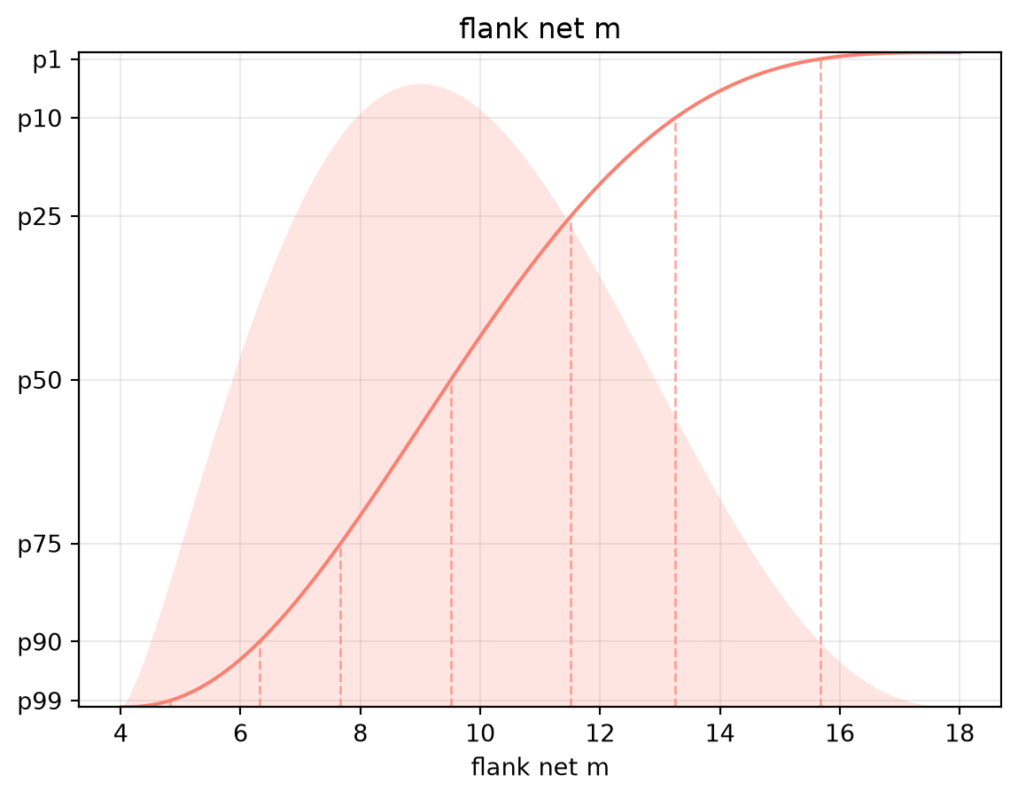

Compose the prospect model

A prospect is just the sum of the risked reservoir models.

prospect = shallow.oil_mmbbl() + deep.oil_mmbbl() + flank.oil_mmbbl()
prospect.name = "STOIIP MMbbl"

Add cross-input correlations

By default, distribution leaves are sampled independently. Use .correlate(...) to add a Gaussian copula across the whole composed model. Here we use:

strong positive correlation on sand success (capturing risk dependency),
weak positive cross-reservoir correlation between porosity variables,
stronger positive correlation between porosity and net pay within each reservoir, and
negative correlations between area and sw within each reservoir.

All other pairwise correlations are left at zero.

def prospect_correlation_matrix(model: dr.MCModel) -> np.ndarray:
    """Build a correlation matrix aligned to model.distributions() order."""
    distributions = model.distributions()
    names = [distribution.name for distribution in distributions]
    correlation = np.eye(len(distributions))

    def set_correlation(left: str, right: str, value: float) -> None:
        i = names.index(left)
        j = names.index(right)
        correlation[i, j] = value
        correlation[j, i] = value

    porosity_names = ["shallow phi", "deep phi", "flank phi"]
    for i, left in enumerate(porosity_names):
        for right in porosity_names[i + 1:]:
            set_correlation(left, right, 0.35)

    success_names = [
        "shallow success", 
        "deep success", 
        "flank success"
    ]
    for i, left in enumerate(success_names):
        for right in success_names[i + 1:]:
            set_correlation(left, right, 0.75)

    set_correlation("shallow phi", "shallow net m", 0.5)
    set_correlation("shallow area km2", "shallow sw", -0.5)
    set_correlation("shallow net m", "shallow sw", -0.5)

    set_correlation("deep phi", "deep net m", 0.5)
    set_correlation("deep area km2", "deep sw", -0.5)
    set_correlation("deep net m", "deep sw", -0.5)

    set_correlation("flank phi", "flank net m", 0.5)
    set_correlation("flank area km2", "flank sw", -0.5)
    set_correlation("flank net m", "flank sw", -0.5)

    return correlation


prospect.correlate(prospect_correlation_matrix(prospect))

# Plot matrix
fig, ax = plt.subplots(figsize=(12, 10))
prospect.copula.corr_matrix.plot(
    labels=[d.name for d in prospect.distributions()],
    ax=ax
)
fig.tight_layout()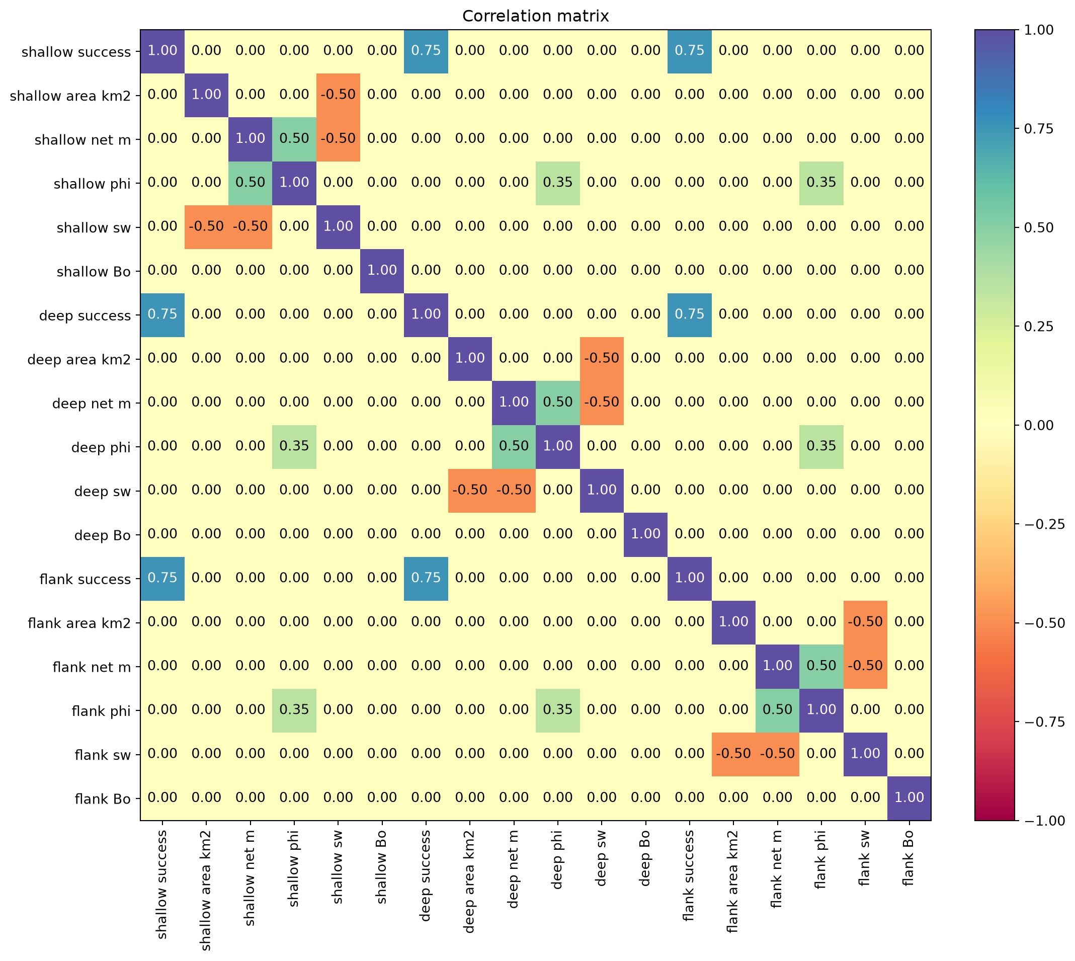

summary = prospect.summary(
    size=50_000, 
    seed=42, 
    threshold=0, 
    conditional_on_threshold=True,
    precision=1
)
summary

	p(> 0)	mean \| > 0	p99 \| > 0	p90 \| > 0	p75 \| > 0	p50 \| > 0	p25 \| > 0	p10 \| > 0	p1 \| > 0
metric
STOIIP MMbbl	0.7	402.3	42.0	100.6	169.9	313.6	543.5	816.2	1504.4

Inspect the result

The distribution has a spike at zero because all reservoirs can fail, with a long upside tail from combinations of success and larger volumetric outcomes.

fig, ax = plt.subplots(figsize=(8, 4.5))
prospect.plot(ax=ax, size=50_000, seed=42, color="green")

ax.set_title("Risked prospect oil in place")
ax.set_xlabel("Oil in place, MMbbl")

fig.tight_layout()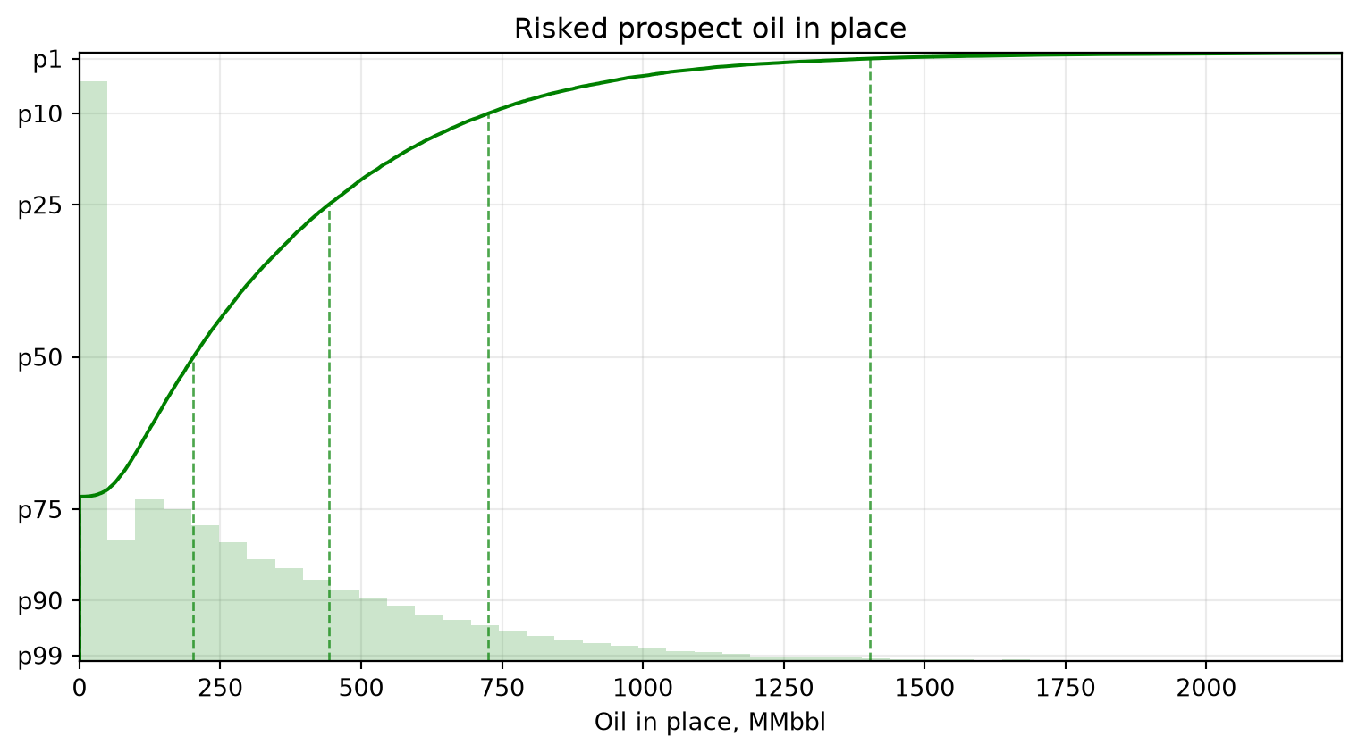

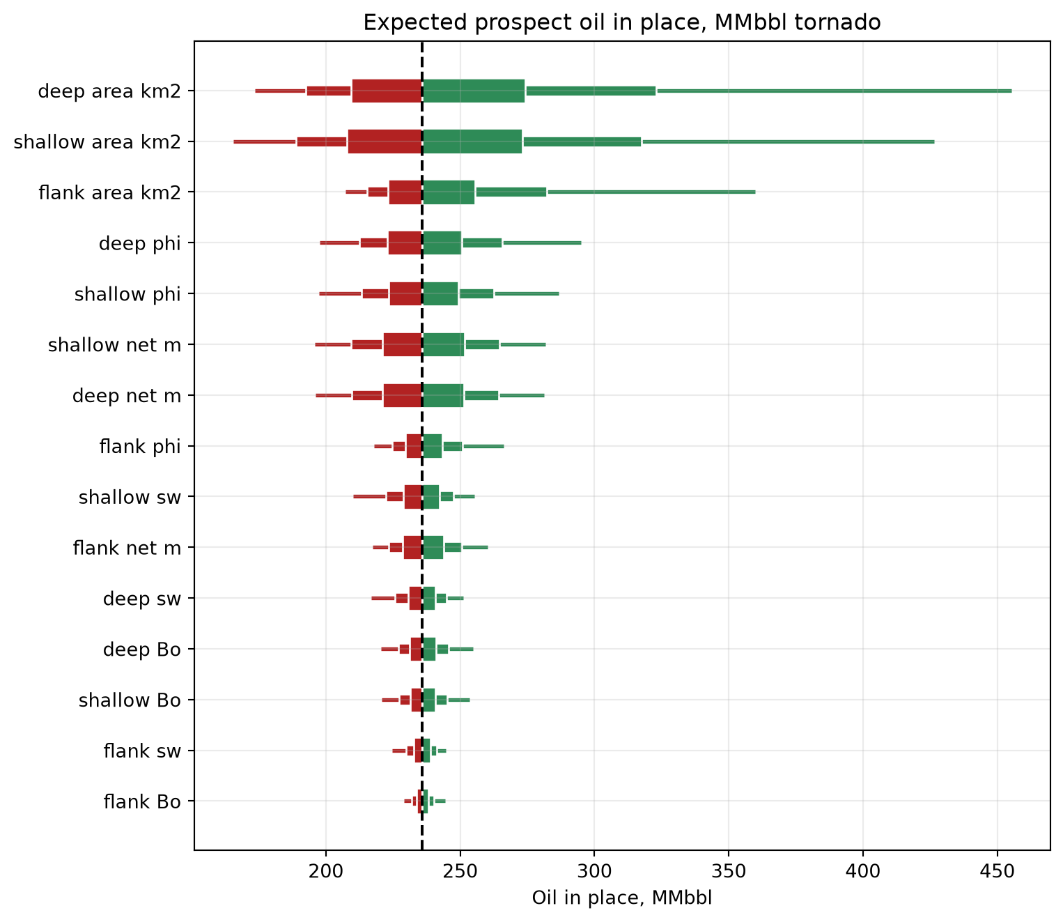
Sensitivity tornado

A one-at-a-time sensitivity tornado helps identify which input distributions drive the median prospect outcome. Each variable is varied through percentile bands while the other inputs are held at their median values. Green bars indicate upside relative to the median result, while red bars indicate downside.

For this example, we plot sensitivity on an expected-value version of the prospect model: each reservoir’s success-case volume is multiplied by its chance of success. This avoids hiding deep and flank volumetric sensitivities when their Bernoulli success variables are fixed at their median failure outcome.

expected_prospect = (
    shallow.expected_oil_mmbbl()
    + deep.expected_oil_mmbbl()
    + flank.expected_oil_mmbbl()
)
expected_prospect.name = "Expected prospect oil in place, MMbbl"

fig, ax = plt.subplots(figsize=(8, 7))
expected_prospect.plot_sensitivity(ax=ax)

ax.set_xlabel("Oil in place, MMbbl")
fig.tight_layout()