Decision Trees for Business Decisions

Rollback analysis with uncertain outcomes

Motivation

Decision trees are useful when a business choice is followed by uncertain events. In drisk, DecisionNode, ChanceNode, and OutcomeNode mirror traditional decision tree notation while still accepting ordinary drisk distributions and MCModel expressions as uncertain values.

This example evaluates whether to drill an exploration well. The decision maker can choose to drill or walk away. If they drill, the reservoir can be a success or a dry hole. A successful discovery then creates a second decision: whether to develop the field. The developed-field value is uncertain and represented by a lognormal distribution.

import matplotlib.pyplot as plt
import numpy as np

import drisk as dr

Define uncertain outcomes

The developed-field value is positive and right-skewed, so we model it as a lognormal distribution elicited from an 80% confidence interval. Drilling cost is included in the terminal NPVs as an up-front cost incurred before the reservoir outcome resolves.

drill_cost = 8_000_000

developed_field_value = dr.LogNormal.elicit(
    lower=35_000_000,
    upper=90_000_000,
    confidence=0.8,
    name="Developed field value",
)

develop_npv = developed_field_value - drill_cost
develop_outcome = dr.OutcomeNode(develop_npv, name="Develop NPV")
do_not_develop_outcome = dr.OutcomeNode(-drill_cost, name="Do not develop NPV")
dry_hole_outcome = dr.OutcomeNode(-drill_cost, name="Dry hole NPV")

An OutcomeNode can contain an MCModel, not just a scalar. Here the develop outcome is itself uncertain because it is based on the lognormal developed-field value.

fig, ax = plt.subplots(figsize=(8, 4.5))

dr.DTree(develop_outcome, name="Develop outcome").plot(
    ax=ax,
    size=50_000,
    seed=42,
    color="#4C78A8",
)

ax.axvline(0, color="black", linestyle="--", linewidth=1, label="Break-even")
ax.set_title("CDF for the uncertain develop outcome")
ax.set_xlabel("NPV")
ax.legend()
fig.tight_layout()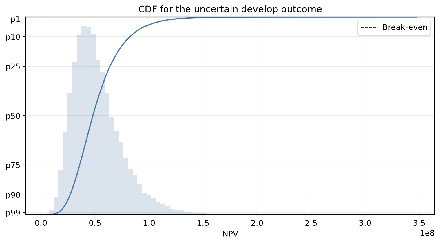

Build the decision tree

The compact dictionary API keeps the tree close to the business diagram:

• decision branches map branch name to the next node or outcome;
• chance branches map branch name to (probability, next node or outcome).

tree = dr.DTree(
    name="Exploration decision",
    root=dr.DecisionNode(
        "Drill exploration well?",
        {
            "Drill": dr.ChanceNode(
                "Exploration outcome",
                {
                    "Discovery": (
                        0.75,
                        dr.DecisionNode(
                            "Develop field?",
                            {
                                "Develop": develop_outcome,
                                "Do not develop": do_not_develop_outcome,
                            },
                        ),
                    ),
                    "Dry hole": (
                        0.25, 
                        dry_hole_outcome
                    ),
                },
            ),
            "Walk": 0,
        },
    ),
)

Visualize the tree

plot_tree() draws the tree from top to bottom using conventional business decision-tree shapes: green squares for decisions, maroon circles for chance nodes, and blue triangles for outcomes.

fig, ax = plt.subplots(figsize=(16, 12))
tree.plot_tree(ax=ax, size=50_000, seed=42, precision=0)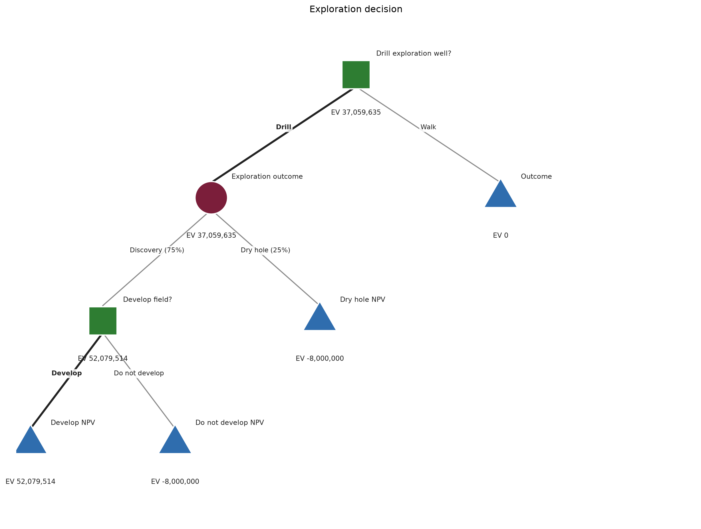

Roll back the tree

Rollback computes expected values from the terminal outcomes back to the root and marks the selected branch at decision nodes. Decision sampling later follows this selected policy; it does not choose the best branch sample-by-sample with perfect information.

rollback = tree.rollback(size=50_000, seed=42, precision=0)
rollback

	node_type	branch	probability	expected_value	selected
node
Drill exploration well?	decision	Drill	NaN	37059635.0	True
Drill exploration well?	decision	Walk	NaN	0.0	False
Develop field?	decision	Develop	NaN	52079514.0	True
Develop field?	decision	Do not develop	NaN	-8000000.0	False

Simulate the selected policy

After rollback selects a decision branch, sample() simulates actual outcomes under that policy. Chance nodes route samples according to their branch probabilities, and uncertain outcome values are sampled using the same Monte Carlo machinery as any other drisk model.

summary = tree.summary(size=50_000, seed=123, percentiles=(90, 50, 10), precision=0)
summary

	mean	p90	p50	p10
metric
Exploration decision	37061810.0	-8000000.0	39873471.0	76116695.0

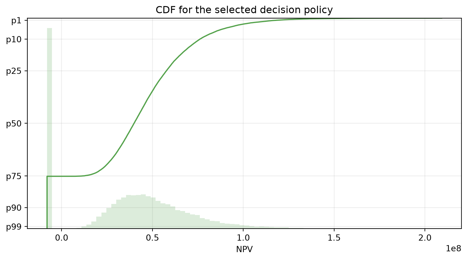
samples = tree.sample(size=50_000, seed=123)
prob_loss = np.mean(samples < 0)
print(f"Probability of loss under selected policy: {prob_loss:.1%}")

Probability of loss under selected policy: 24.9%

fig, ax = plt.subplots(figsize=(8, 4.5))
tree.plot(ax=ax, size=50_000, seed=123, color="#54A24B")
ax.set_title("CDF for the selected decision policy")
ax.set_xlabel("NPV")
fig.tight_layout()